vignette_ebpm2

EBPM problem

\[ \begin{align} & x_i \sim Pois(s_i \lambda_i)\\ & \lambda_i \sim g(.)\\ & g \in \mathcal{G} \end{align} \] Our goal is to estimate \(\hat{g}\) (MLE), then compute posterior \(p(\lambda_i | x_i, \hat{g})\). Here I use point gamma (spike-and-slab) as prior family.

See model details and derivations in https://github.com/stephenslab/ebpm/blob/master/derivations/ebpm.pdf

devtools::load_all("../ebpm")

Loading ebpm

set.seed(123)
library(ebpm)
library(ggplot2)
library(gtools)
require(gridExtra)

Loading required package: gridExtra

experiment setup

I simulate data from the mixture of exponential, and compare fitting the poisson mean problem with MLE (\(\hat{\lambda}^{mle}_i = \frac{x_i}{s_i}\)), and ebpm_exponential_mixture with different options.
For ebpm, the options are: * fit_true_g: use the true \(g\)
* fit_true_scale: use the true mixture components to estimate \(\hat{g}\) * fit_est_scale: estimate mixture components from data, then estimate \(\hat{g}\)

## simulate data
n = 20000
sim = ebpm::simulate_pois_point_gamma(n, g_init = point_gamma(0.4,1,1))
hist(log(sim$x+1), breaks = 100, xlab = "log(x + 1)", main = "hist for log(x + 1)")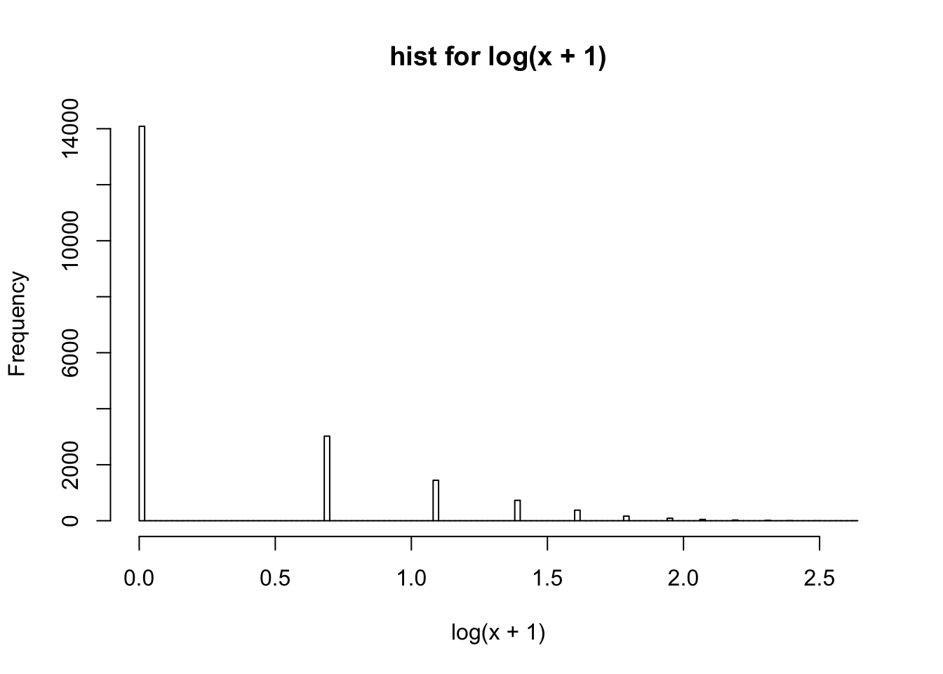

rmse <- function(x,y){
  return(sqrt(mean((x-y)^2)))
}
methods = c()
ll_gs = c()
rmses = c()
## true
methods = c(methods, "true")
ll_gs = c(ll_gs, sim$ll)
rmses = c(rmses, 0)

## MLE
methods = c(methods, "mle")
ll_gs = c(ll_gs, NA)
rmses = c(rmses, rmse(sim$x/sim$s, sim$lam))


## fit (with known g)
fit = ebpm::ebpm_point_gamma(x = sim$x, s = sim$s, g_init = sim$g, fix_g = T)
methods = c(methods, "fit_true_g")
ll_gs = c(ll_gs, fit$log_likelihood)
rmses = c(rmses, rmse(fit$posterior$mean, sim$lam))
rm(fit)


## fit (estimate scale)
fit = ebpm::ebpm_point_gamma(x = sim$x, s = sim$s)
methods = c(methods, "fit_est_g")
ll_gs = c(ll_gs, fit$log_likelihood)
rmses = c(rmses, rmse(fit$posterior$mean, sim$lam))
rm(fit)

data.frame(method = methods, ll_g = ll_gs, rmse = rmses)

      method      ll_g      rmse
1       true -20247.31 0.0000000
2        mle        NA 0.7742208
3 fit_true_g -20247.31 0.5822832
4  fit_est_g -20245.22 0.5824073

plot the \(\lambda\)s

fit = ebpm::ebpm_point_gamma(x = sim$x, s = sim$s)
df = data.frame(lam_true = sim$lam,lam_hat_mle = sim$x/sim$s, lam_hat_ebpm = fit$posterior$mean)
ggplot(df)+
  geom_point(aes(x = log(lam_true + 1), y = log(lam_hat_ebpm +1)), color = "blue")+
  geom_abline(slope = 1, intercept = 0)+
  guides(fill = "color")+
  ggtitle("lam_true vs lam_hat_ebpm")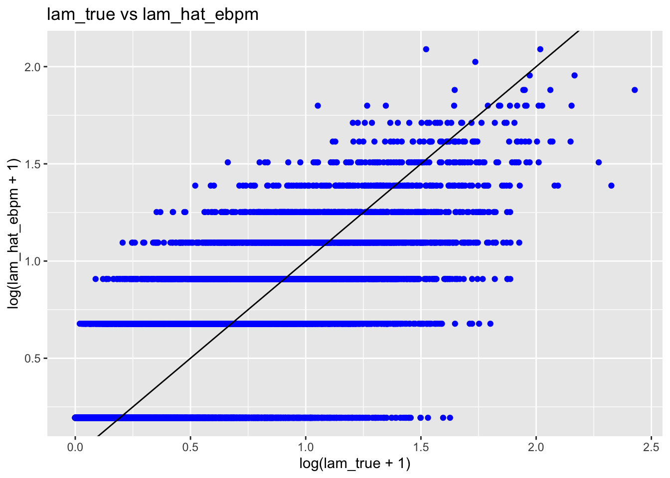

ggplot(df)+
  geom_point(aes(x = log(lam_true + 1), y = log(lam_hat_mle + 1)), color = "blue")+
  geom_abline(slope = 1, intercept = 0)+
  guides(fill = "color")+
  ggtitle("lam_true vs lam_hat_mle")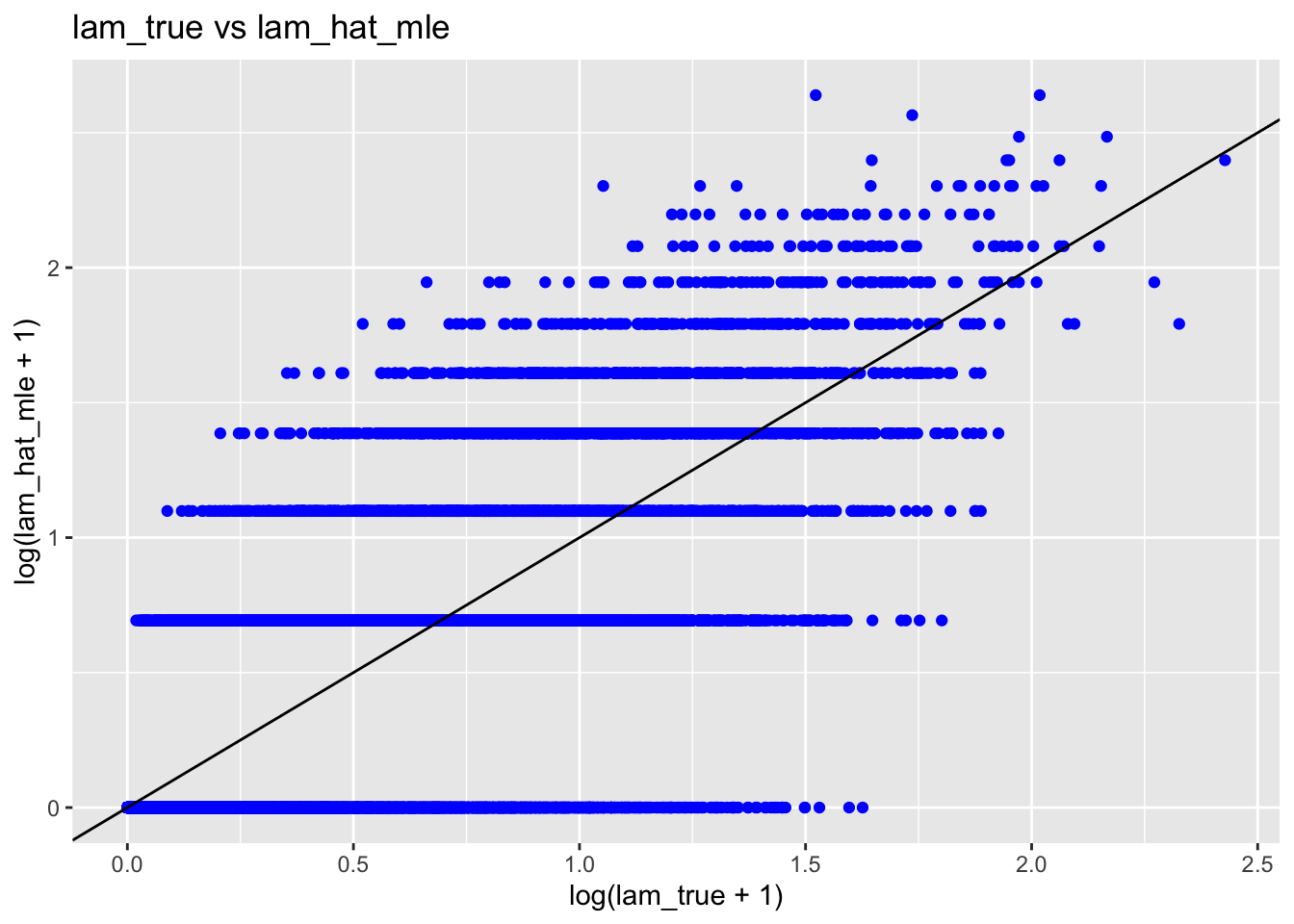

ggplot(df)+
  geom_point(aes(x = log(lam_hat_mle + 1), y = log(lam_hat_ebpm + 1)), color = "blue")+
  geom_abline(slope = 1, intercept = 0)+
  guides(fill = "color")+
  ggtitle("lam_hat_mle vs lam_hat_ebpm")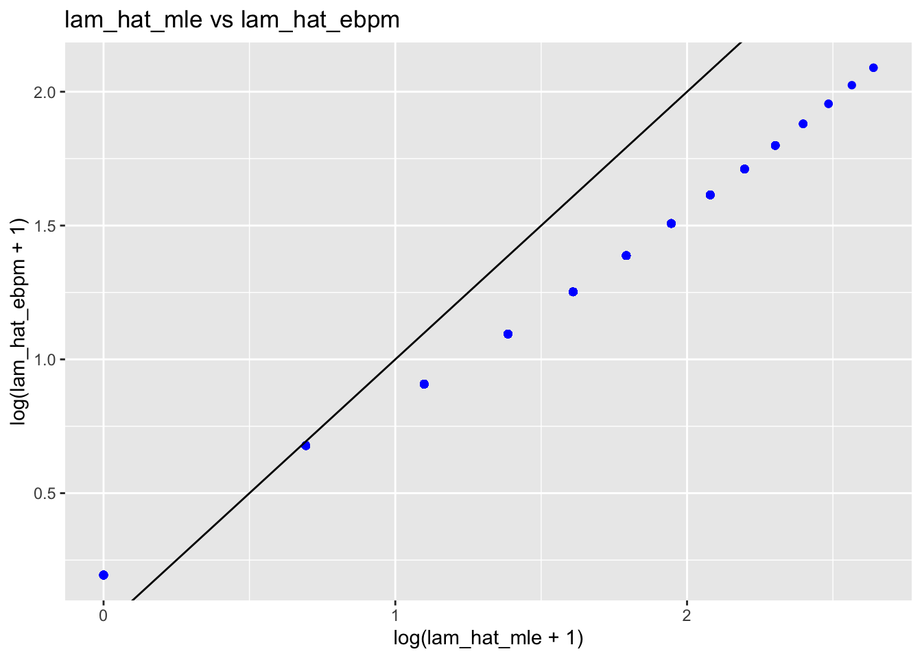

With outliers

What if there are outliers in our data? I add a few very numbers to the original data. Let’s see what will ebpm and MLE give us:

n_outlier = 10
sim2 = sim
sim2$x = c(sim2$x, runif(n_outlier, 1e+4, 1e+5))
sim2$s = c(sim$s, replicate(n_outlier, 1))

fit2 = ebpm::ebpm_point_gamma(x = sim$x, s = sim$s)

## MLE estimate
tail(sim2$x/sim2$s, n_outlier)

 [1] 82892.51 66284.71 36595.39 95580.53 98246.45 57903.75 99663.95
 [8] 46440.66 32593.94 26183.92

## `ebpm` estimate
tail(fit2$posterior$mean, n_outlier)

 [1] 0.2140541 0.2140541 0.2140541 2.4975590 0.9693591 0.2140541 0.2140541
 [8] 0.2140541 0.2140541 0.2140541

So ebpm shrinks those abnormally big data towards smaller values.

Session information

sessionInfo()

R version 3.5.1 (2018-07-02)
Platform: x86_64-apple-darwin15.6.0 (64-bit)
Running under: macOS  10.14

Matrix products: default
BLAS: /Library/Frameworks/R.framework/Versions/3.5/Resources/lib/libRblas.0.dylib
LAPACK: /Library/Frameworks/R.framework/Versions/3.5/Resources/lib/libRlapack.dylib

locale:
[1] en_US.UTF-8/en_US.UTF-8/en_US.UTF-8/C/en_US.UTF-8/en_US.UTF-8

attached base packages:
[1] stats     graphics  grDevices utils     datasets  methods   base     

other attached packages:
[1] gridExtra_2.3   gtools_3.8.1    ggplot2_3.2.1   ebpm_0.0.0.9001
[5] testthat_2.2.1 

loaded via a namespace (and not attached):
 [1] Rcpp_1.0.2          pillar_1.4.2        compiler_3.5.1     
 [4] git2r_0.25.2        workflowr_1.4.0     prettyunits_1.0.2  
 [7] remotes_2.1.0       tools_3.5.1         digest_0.6.21      
[10] pkgbuild_1.0.3      pkgload_1.0.2       tibble_2.1.3       
[13] gtable_0.3.0        evaluate_0.14       memoise_1.1.0      
[16] pkgconfig_2.0.3     rlang_0.4.0         cli_1.1.0          
[19] rstudioapi_0.10     yaml_2.2.0          xfun_0.8           
[22] dplyr_0.8.1         withr_2.1.2         stringr_1.4.0      
[25] knitr_1.25          desc_1.2.0          fs_1.3.1           
[28] devtools_2.2.1.9000 tidyselect_0.2.5    grid_3.5.1         
[31] rprojroot_1.3-2     glue_1.3.1          R6_2.4.0           
[34] processx_3.3.1      rmarkdown_1.13      sessioninfo_1.1.1  
[37] mixsqp_0.1-121      purrr_0.3.2         callr_3.2.0        
[40] magrittr_1.5        scales_1.0.0        backports_1.1.5    
[43] ps_1.3.0            ellipsis_0.3.0      htmltools_0.3.6    
[46] usethis_1.5.1       assertthat_0.2.1    colorspace_1.4-1   
[49] labeling_0.3        stringi_1.4.3       lazyeval_0.2.2     
[52] munsell_0.5.0       crayon_1.3.4