ebpm_point_gamma_demo
zihao12
2019-09-28
Last updated: 2019-10-04
Checks: 7 0
Knit directory: ebpmf_demo/
This reproducible R Markdown analysis was created with workflowr (version 1.4.0). The Checks tab describes the reproducibility checks that were applied when the results were created. The Past versions tab lists the development history.
Great! Since the R Markdown file has been committed to the Git repository, you know the exact version of the code that produced these results.
Great job! The global environment was empty. Objects defined in the global environment can affect the analysis in your R Markdown file in unknown ways. For reproduciblity it’s best to always run the code in an empty environment.
The command set.seed(20190923) was run prior to running the code in the R Markdown file. Setting a seed ensures that any results that rely on randomness, e.g. subsampling or permutations, are reproducible.
Great job! Recording the operating system, R version, and package versions is critical for reproducibility.
Nice! There were no cached chunks for this analysis, so you can be confident that you successfully produced the results during this run.
Great job! Using relative paths to the files within your workflowr project makes it easier to run your code on other machines.
Great! You are using Git for version control. Tracking code development and connecting the code version to the results is critical for reproducibility. The version displayed above was the version of the Git repository at the time these results were generated.
Note that you need to be careful to ensure that all relevant files for the analysis have been committed to Git prior to generating the results (you can use wflow_publish or wflow_git_commit). workflowr only checks the R Markdown file, but you know if there are other scripts or data files that it depends on. Below is the status of the Git repository when the results were generated:
Ignored files:
    Ignored:    .Rhistory
    Ignored:    .Rproj.user/

Untracked files:
    Untracked:  analysis/.ipynb_checkpoints/
    Untracked:  analysis/ebpmf_demo.Rmd
    Untracked:  analysis/softmax_experiments.ipynb
    Untracked:  docs/figure/test.Rmd/

Unstaged changes:
    Modified:   analysis/softmax_experiments.Rmd
Note that any generated files, e.g. HTML, png, CSS, etc., are not included in this status report because it is ok for generated content to have uncommitted changes.
These are the previous versions of the R Markdown and HTML files. If you’ve configured a remote Git repository (see ?wflow_git_remote), click on the hyperlinks in the table below to view them.
| File | Version | Author | Date | Message |
|---|---|---|---|---|
| Rmd | b2852bc | zihao12 | 2019-10-04 | rerun after fixing bug at ebpm |
| html | c677680 | zihao12 | 2019-09-30 | Build site. |
| html | 3dd3e5c | zihao12 | 2019-09-30 | Build site. |
| Rmd | 2c4ab46 | zihao12 | 2019-09-30 | update demo after library changes |
| html | bed7f5c | zihao12 | 2019-09-29 | Build site. |
| Rmd | 7d1822f | zihao12 | 2019-09-29 | add rmse |
| html | 206c292 | zihao12 | 2019-09-29 | Build site. |
| Rmd | 41a62f0 | zihao12 | 2019-09-29 | ebpm_point_gamma_demo |
| html | b1261b1 | zihao12 | 2019-09-29 | Build site. |
| Rmd | 62e5d59 | zihao12 | 2019-09-29 | ebpm_point_gamma_demo |
| html | f5ecee3 | zihao12 | 2019-09-28 | Build site. |
| html | 0df3869 | zihao12 | 2019-09-28 | Build site. |
| Rmd | f7d4408 | zihao12 | 2019-09-28 | demo for point-gamma, with bug |
library(stats)
library(ggplot2)
Warning: package 'ggplot2' was built under R version 3.5.2set.seed(123)Goal
I want to implement the ebpm_point_gamma algortihm, and test it against data generated the same way as described in the model below.
EBPM problem with spike-and-slab prior
\[ \begin{align} & x_i \sim Pois(s_i \lambda_i)\\ & \lambda_i \sim g(.)\\ & g \in \mathcal{G} \end{align} \]
where \(\mathcal{G} = \{\pi_0 \delta(.) + (1-\pi_0) gamma(a,b): \pi_0 \in [0,1] \}\)
Now the goal is to compute \(\hat{\pi}_0,\hat{a}, \hat{b}\) with MLE, then compute posterior mean of \(\lambda_i\).
MLE
\[ \begin{align} & l(\pi_0, a, b) = \sum_i log \{\pi_0 c_i(a, b) + d_i(a, b) \}\\ & d_i(a, b) := NB(x_i, a, \frac{b}{b + s})\\ & c_i := \delta(x_i) - d_i(a,b) \end{align} \] #### functions for optimization in “nlm”
pg_nlm_fn <- function(par, x, s){
  pi = 1/(1+ exp(-par[1]))
  a = exp(par[2])
  b  =  exp(par[3])
  d <- dnbinom(x, a, b/(b+s), log = F)
  c = as.integer(x ==  0) - d
  return(-sum(log(pi*c + d)))
}

transform_param <- function(par0){
  par = rep(0,length(par0))
  par[1] = log(par0[1]/(1-par0[1]))
  par[2] = log(par0[2])
  par[3] = log(par0[3])
  return(par)
}

transform_param_back <- function(par){
  par0 = rep(0,length(par))
  #par0[1] = log(par[1]) - log(1-par[1])
  par0[1] = 1/(1+ exp(-par[1]))
  par0[2] = exp(par[2])
  par0[3] = exp(par[3])
  return(par0)
}
sim_spike_one <- function(pi, a, b){
if(rbinom(1,1, pi)){return(0)}
else{return(rgamma(1,shape = a, rate = b))}
}
simulate_pm <- function(s, param){
pi = param[1]
a = param[2]
b = param[3]
lam = replicate(length(s), sim_spike_one(pi, a, b))
x = rpois(length(s), s*lam)
ll = -pg_nlm_fn(transform_param(param), x, s)
return(list(x = x, s= s, lam = lam, param = param, ll = ll))
}n = 4000
s = replicate(n, 1)
pi = 0.8
a = 100
b = 1
param = c(pi, a, b)
sim = simulate_pm(s, param)init_par = c(0.5,1,1)
opt = nlm(pg_nlm_fn, transform_param(init_par), sim$x, sim$s)
opt_par = transform_param_back(opt$estimate)[1] "oracle ll: -5166.363892"[1] "opt ll: -5165.270752"[1] "oracle:pi, a, b"[1] 0.8 100.0 1.0[1] "estimate: pi, a, b"[1] 0.80 107.79 1.08Comment:
- Estimated parameter gets better loglikelihood than oracle, and is similar to oracle (in a sense).
- However, there are some warnings in the process.
- To do: add gradient and Hessian
Wrap up into ebpm algorithm
It is easy to deduce posterior mean:
\[ \begin{align} \text{posterior mean} = \frac{(1-\pi_0)NB(x; a, \frac{b}{b + s}) \frac{a+x}{b+s}}{\pi_0 \delta(x) + (1-\pi_0)NB(x; a , \frac{b}{b + s})} \end{align} \]
ebpm_point_gamma_demo <- function(x, s, init_par = c(0.5,1,1), seed = 123){
  set.seed(seed) ## though seems determined
  ## MLE
  opt = nlm(pg_nlm_fn, transform_param(init_par), x, s)
  opt_par = transform_param_back(opt$estimate)
  ll =  -pg_nlm_fn(transform_param(opt_par), x, s)

  ## posterior mean
  pi = opt_par[1]
  a =  opt_par[2]
  b =  opt_par[3]
  nb = dnbinom(x, size = a, prob = b/(b+s))
  pm = ((1-pi)*nb*(a+x)/(b+s))/(pi*as.integer(x ==  0) + (1-pi)*nb)
  return(list(param = opt_par, lam_pm = pm, ll = ll))
}
I have packaged the functions above into the ebpm package functin ebpm_point_gamma. Try it out!
library(ebpm)
start = proc.time()
fit <- ebpm_point_gamma(sim$x, sim$s)
Called from: f(x, ...)
debug at /Users/ontheroad/Desktop/git/ebpm/R/ebpm_point_gamma.R#61: return(-sum(log(pi * c + d)))
[1] 1.40673212 4.68017717 0.08098415runtime = proc.time() - start
print(sprintf("fit %d data with runtime %f seconds", n, runtime[[3]]))[1] "fit 4000 data with runtime 0.128000 seconds"Compare RMSE with \(\lambda_{oracle}\)
[1] "RMSE with lam_oracle:"[1] "mle : 4.204930"[1] "fitted : 3.041565"df <- data.frame(n = 1:length(sim$x), x = sim$x, s = sim$s, lam = sim$lam, lam_pm = fit$posterior$mean)
ggplot(df) + geom_point(aes(x = x/s, y = lam_pm), color = "blue", cex = 0.5) +
labs(x = "x/s", y = "lam_pm", title = "ebpm_point_gamma: x/s vs lam_posterior_mean") +
guides(fill = "color")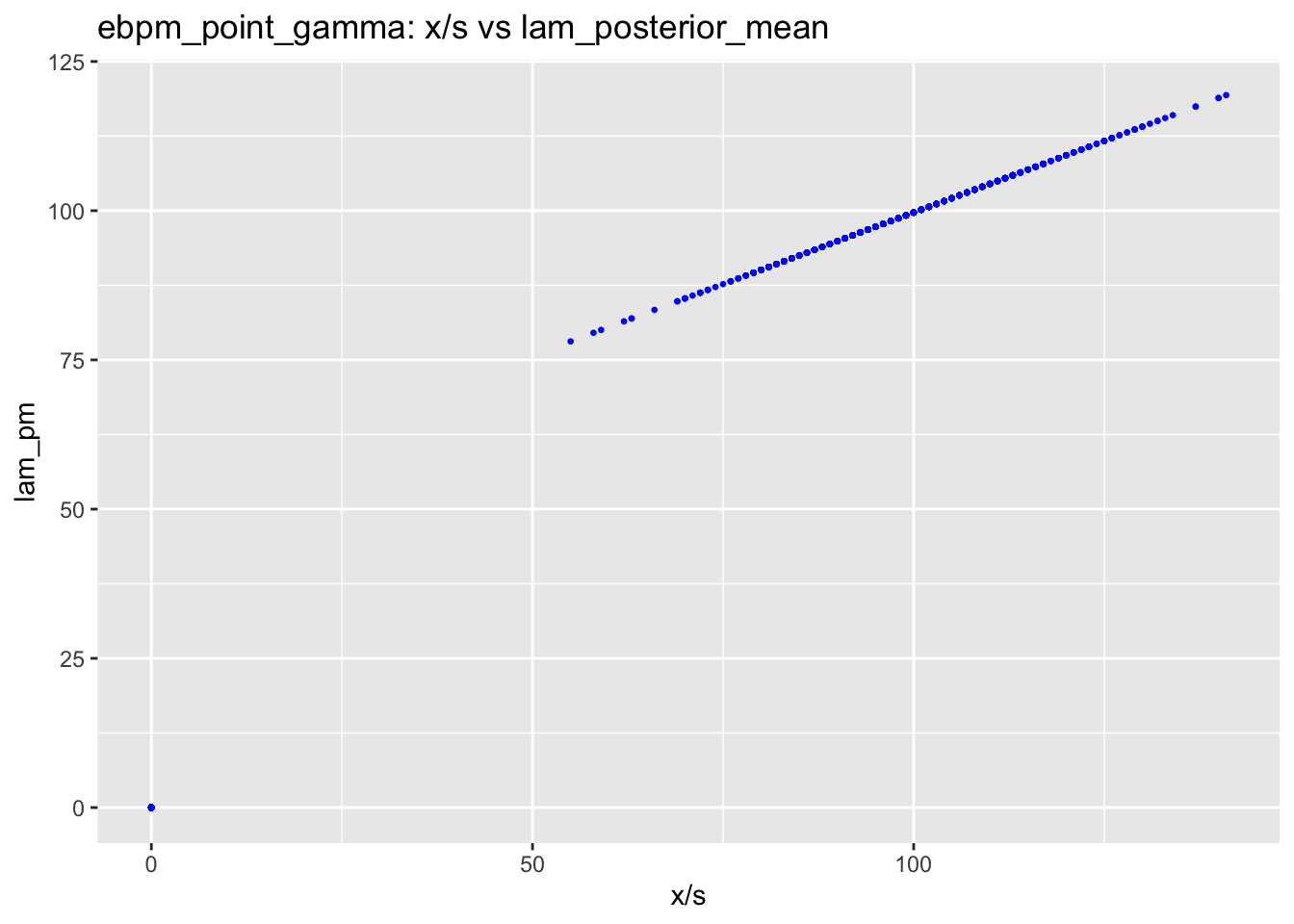
| Version | Author | Date |
|---|---|---|
| bed7f5c | zihao12 | 2019-09-29 |
[1] "max posterior mean when x = 0"[1] 3.251273e-30Let’s take a look at the nonzero (for x) parts.
Note that for \(x \neq 0\), we have posterior mean \(\frac{a+x}{b+s}\). Therefore we expect to see a line, with slope \(1/(1 + \frac{b}{s})\)
df_nz = df[df$x != 0, ]
ggplot(df_nz)  + geom_point(aes(x = x/s, y = lam_pm), color = "blue", cex = 0.5) +
    labs(x = "x/s", y = "lam_pm", title = "ebpm_point_gamma: x/s vs lam_posterior_mean") +
    geom_abline(slope = 1, intercept = 0)+
    guides(fill = "color")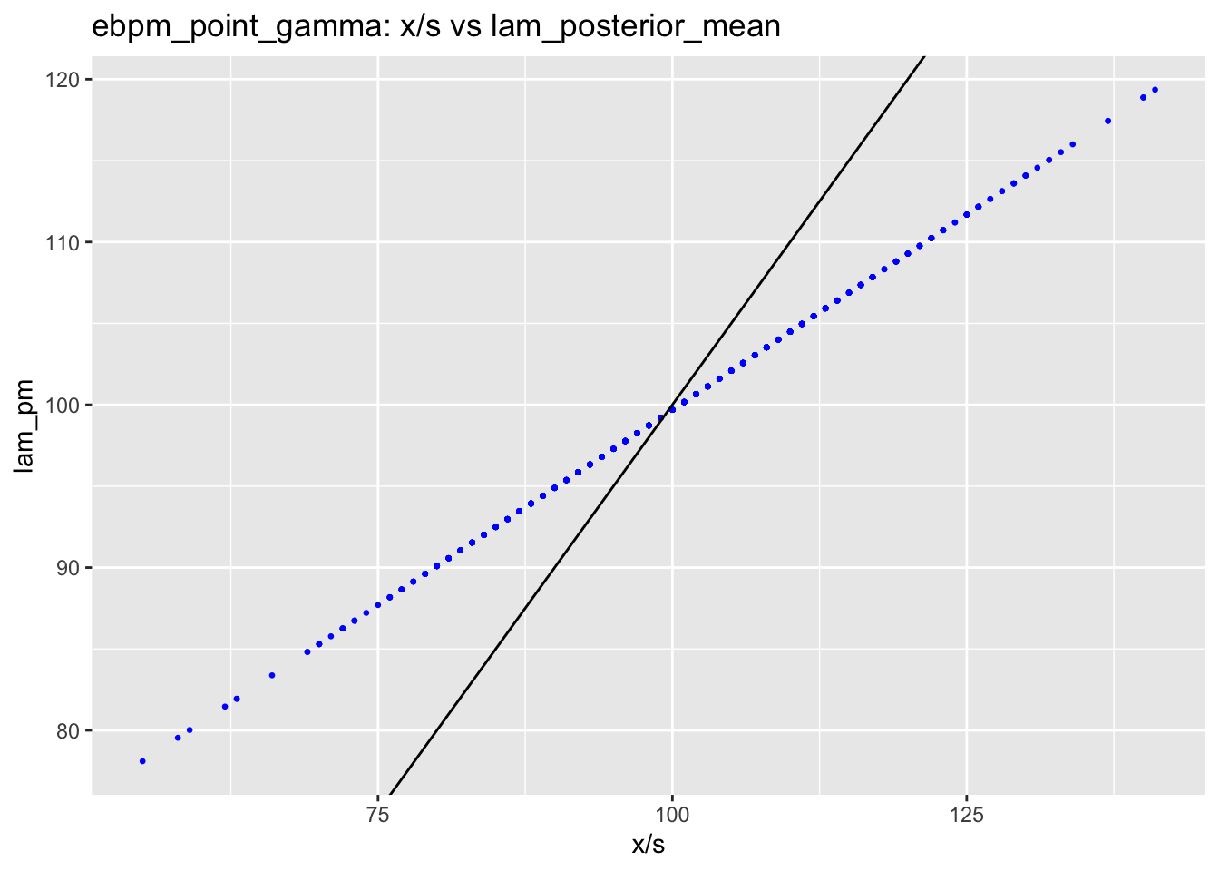
now let’s compare \(\lambda_{true}, \lambda_{\text{posterior mean}}\)
ggplot(df_nz)  + geom_point(aes(x = lam, y = lam_pm), color = "blue", cex = 0.5) +
    labs(x = "lam_true", y = "lam_pm", title = "ebpm_point_gamma: lam _true lam_posterior_mean") +
    geom_abline(slope = 1, intercept = 0)+
    guides(fill = "color")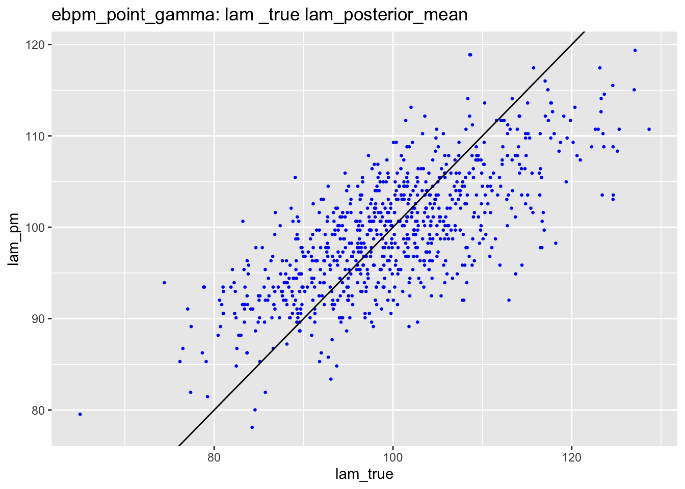
| Version | Author | Date |
|---|---|---|
| bed7f5c | zihao12 | 2019-09-29 |
sessionInfo()R version 3.5.1 (2018-07-02)
Platform: x86_64-apple-darwin15.6.0 (64-bit)
Running under: macOS 10.14
Matrix products: default
BLAS: /Library/Frameworks/R.framework/Versions/3.5/Resources/lib/libRblas.0.dylib
LAPACK: /Library/Frameworks/R.framework/Versions/3.5/Resources/lib/libRlapack.dylib
locale:
[1] en_US.UTF-8/en_US.UTF-8/en_US.UTF-8/C/en_US.UTF-8/en_US.UTF-8
attached base packages:
[1] stats graphics grDevices utils datasets methods base
other attached packages:
[1] ebpm_0.0.0.9000 ggplot2_3.2.1
loaded via a namespace (and not attached):
[1] Rcpp_1.0.2 knitr_1.25 whisker_0.3-2 magrittr_1.5
[5] workflowr_1.4.0 tidyselect_0.2.5 munsell_0.5.0 colorspace_1.4-1
[9] R6_2.4.0 rlang_0.4.0 dplyr_0.8.1 stringr_1.4.0
[13] tools_3.5.1 grid_3.5.1 gtable_0.3.0 xfun_0.8
[17] withr_2.1.2 git2r_0.25.2 htmltools_0.3.6 assertthat_0.2.1
[21] yaml_2.2.0 lazyeval_0.2.2 rprojroot_1.3-2 digest_0.6.21
[25] tibble_2.1.3 crayon_1.3.4 mixsqp_0.1-120 purrr_0.3.2
[29] fs_1.3.1 glue_1.3.1 evaluate_0.14 rmarkdown_1.13
[33] labeling_0.3 stringi_1.4.3 pillar_1.4.2 compiler_3.5.1
[37] scales_1.0.0 backports_1.1.5 pkgconfig_2.0.3