Issue_ebpmf

Last updated: 2019-10-12

Checks: 7 0

Knit directory: ebpmf_demo/

This reproducible R Markdown analysis was created with workflowr (version 1.4.0). The Checks tab describes the reproducibility checks that were applied when the results were created. The Past versions tab lists the development history.

R Markdown file: up-to-date

Great! Since the R Markdown file has been committed to the Git repository, you know the exact version of the code that produced these results.

Environment: empty

Great job! The global environment was empty. Objects defined in the global environment can affect the analysis in your R Markdown file in unknown ways. For reproduciblity it’s best to always run the code in an empty environment.

Seed: set.seed(20190923)

The command set.seed(20190923) was run prior to running the code in the R Markdown file. Setting a seed ensures that any results that rely on randomness, e.g. subsampling or permutations, are reproducible.

Session information: recorded

Great job! Recording the operating system, R version, and package versions is critical for reproducibility.

Cache: none

Nice! There were no cached chunks for this analysis, so you can be confident that you successfully produced the results during this run.

File paths: relative

Great job! Using relative paths to the files within your workflowr project makes it easier to run your code on other machines.

Repository version: c3ecc2c

Great! You are using Git for version control. Tracking code development and connecting the code version to the results is critical for reproducibility. The version displayed above was the version of the Git repository at the time these results were generated.

Note that you need to be careful to ensure that all relevant files for the analysis have been committed to Git prior to generating the results (you can use wflow_publish or wflow_git_commit). workflowr only checks the R Markdown file, but you know if there are other scripts or data files that it depends on. Below is the status of the Git repository when the results were generated:


Ignored files:
    Ignored:    .Rhistory
    Ignored:    .Rproj.user/

Untracked files:
    Untracked:  analysis/.ipynb_checkpoints/
    Untracked:  analysis/ebpmf_demo.Rmd
    Untracked:  analysis/ebpmf_rank1_demo2.Rmd
    Untracked:  analysis/softmax_experiments.ipynb
    Untracked:  data/trash/
    Untracked:  docs/figure/Experiment_ebpmf_rankk.Rmd/
    Untracked:  docs/figure/test.Rmd/

Unstaged changes:
    Modified:   analysis/ebpmf_rank1_demo.Rmd
    Modified:   analysis/ebpmf_rankk_demo.Rmd
    Modified:   analysis/softmax_experiments.Rmd

Note that any generated files, e.g. HTML, png, CSS, etc., are not included in this status report because it is ok for generated content to have uncommitted changes.

These are the previous versions of the R Markdown and HTML files. If you’ve configured a remote Git repository (see ?wflow_git_remote), click on the hyperlinks in the table below to view them.

File	Version	Author	Date	Message
Rmd	c3ecc2c	zihao12	2019-10-12	Issue_ebpmf_issue2.Rmd
html	244ee32	zihao12	2019-10-12	Build site.
Rmd	d42555c	zihao12	2019-10-12	Issue_ebpmf_issue2.Rmd
Rmd	74fb51c	zihao12	2019-10-12	issues

library(ebpmf)
library(gtools)
library(NNLM)

Goal

I encountered two issues in my experiments for ebpmf (https://github.com/stephenslab/ebpmf), and I reproduce them here:
* ELBO is not montonically increasing (and even decreasing). Either my ELBO formula is wrong, or my algorithm has a bug (it maximizes ELBO using coordinate descent, so should increase in each step). But the trend for RMSE (compare our posterior estimate for \(\Lambda\) with the true one) is decreasing (though there are small exceptions).
* In simulated dataset(simulate from a mixture of gamma), ebpmf methods get much better validation likelihood and RMSE. However, in real 10x genomics dataset, it is getting much worse result on validation set. (\(X\) is the real data. \(Y^{train}_{ij} \sim Bin(0.5, X_{ij})\) and \(Y^{val}_{ij} = X_{ij} - Y^{train}_{ij}\)).

dataset

10X genomics dataset

X = read.csv("data/10xgenomics/cd14_monocytes/filtered_matrices_mex/hg19/Y.csv")
Y = read.csv("data/10xgenomics/cd14_monocytes/filtered_matrices_mex/hg19/Yhat.csv")
real = list(X = as.matrix(X), Y = as.matrix(Y))
print(dim(real$X))

[1] 2611  359

hist(real$X, breaks = 100, main = "hist for Y_train")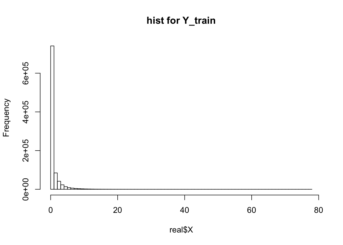

Version	Author	Date
244ee32	zihao12	2019-10-12

simulated dataset

sim_mgamma <- function(dist){
  pi = dist$pi
  a = dist$a
  b = dist$b
  idx = which(rmultinom(1,1,pi) == 1)
  return(rgamma(1, shape = a[idx], rate =  b[idx]))
}

## simulate a poisson mean problem
## to do:
simulate_pm  <-  function(n, p, dl, df, K,scale_b = 10, seed = 123){
  set.seed(seed)
  ## simulate L
  a = replicate(dl,1)
  b = 10*runif(dl)
  pi <- rdirichlet(1,rep(1/dl, dl))
  gl = list(pi = pi, a = a, b= b)
  L = matrix(replicate(n*K, sim_mgamma(gl)), ncol = K)
  ## simulate F
  a = replicate(df,1)
  b = 10*runif(df)
  pi <- rdirichlet(1,rep(1/df, df))
  gf = list(pi = pi, a = a, b= b)
  F = matrix(replicate(p*K, sim_mgamma(gf)), ncol = K)
  ## simulate X
  lam = L %*% t(F)
  X = matrix(rpois(n*p, lam), nrow = n)
  Y = matrix(rpois(n*p, lam), nrow = n)
  ## prepare output
  g = list(gl = gl, gf = gf)
  out = list(X = X, Y = Y, L = L, F = F, g = g)
  return(out)
}

n = 50
p = 100
K = 2
dl = 10
df = 10
scale_b = 5
sim = simulate_pm(n, p, dl, df, K, scale_b = scale_b, seed =12)
print(dim(sim$X))

[1]  50 100

hist(sim$X, breaks = 100, main = "hist for Y_train")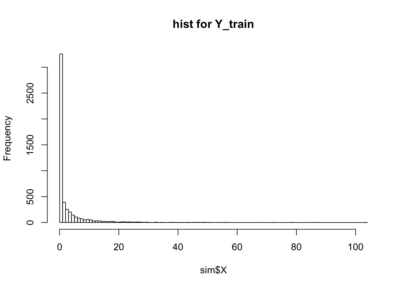

Version	Author	Date
244ee32	zihao12	2019-10-12

ELBOs and RMSE

I cannot get a strictly increasing ELBO. Either the ELBO is wrong, or my algorithm is wrong. Then I check to see if RMSE with true \(\Lambda\) is decreasing, and it seems to.

ELBO and KL

Note the KL is \(KL(q_L || g_L) + KL(q_F || g_F)\). Detail in write up.

`ebpmf_exponential_mixture`

m = 2
out_ebpmf_exp = ebpmf::ebpmf_exponential_mixture(sim$X, K, m = m, maxiter.out = 100)
plot(out_ebpmf_exp$ELBO, type = "l", xlab = "niter", ylab = "ELBO")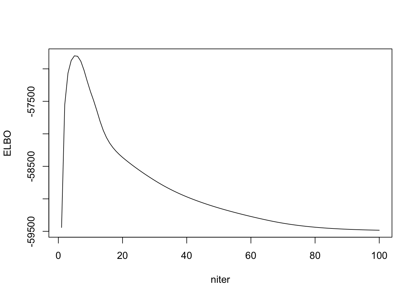

Version	Author	Date
244ee32	zihao12	2019-10-12

plot(out_ebpmf_exp$KL, type = "l", xlab = "niter", ylab = "KL")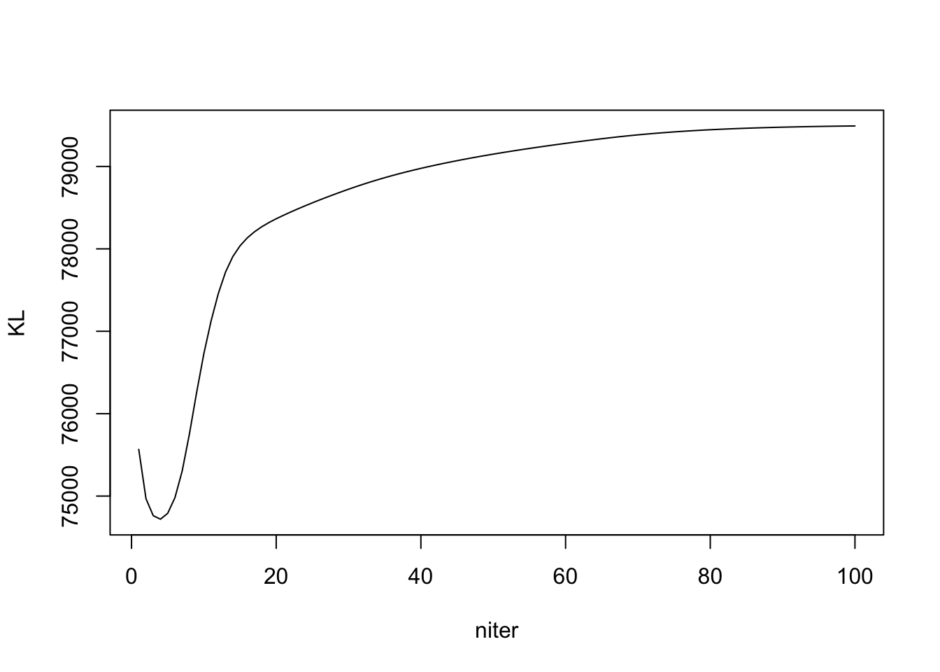

Version	Author	Date
244ee32	zihao12	2019-10-12

## experiment to see RMSE on Lambda
Lam_true = sim$L %*% t(sim$F)
try_experiment_rmse <- function(iter, Lam_true){
  test = ebpmf::ebpmf_exponential_mixture(sim$X, K, m = m, maxiter.out = iter)
  Lam = test$qg$qls_mean %*% t(test$qg$qfs_mean)
  return(sqrt(mean((Lam - Lam_true)^2)))
}

iters = seq(10,100,10)
rmses <- c()
for(iter in iters){
  rmse = try_experiment_rmse(iter, Lam_true)
  rmses = c(rmses, rmse)
}
rmses

 [1] 1.6556401 0.6290973 0.6228208 0.6200187 0.6181718 0.6169139 0.6169600
 [8] 0.6168247 0.6166842 0.6166540

plot(iters, rmses - min(rmses), main  = "distance to smallest rmse", xlab = "iter", type = "l")
points(iters, rmses - min(rmses))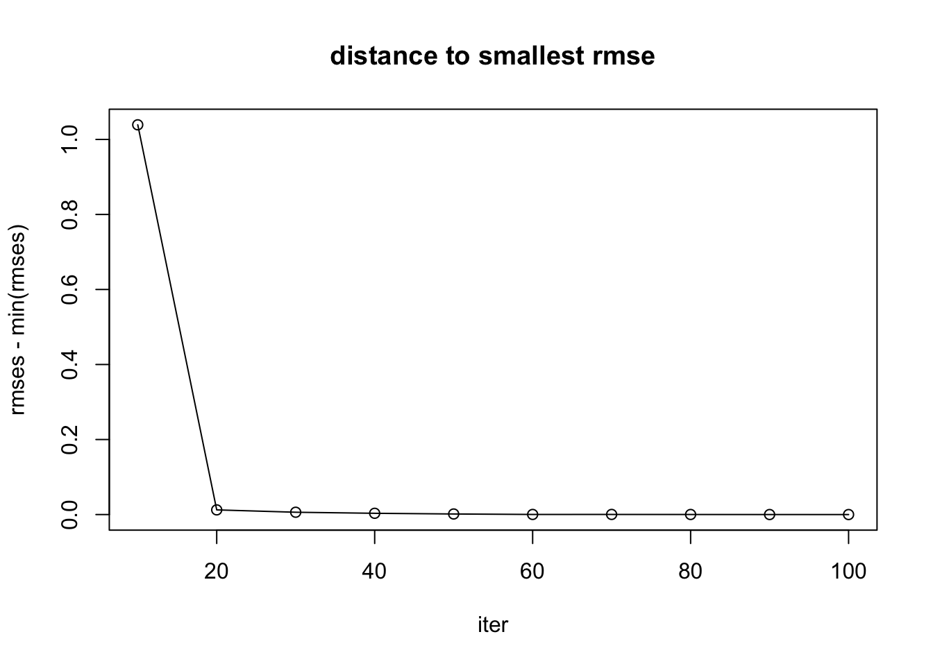

Version	Author	Date
244ee32	zihao12	2019-10-12

`ebpmf_exponential_mixture`

out_ebpmf_exp = ebpmf::ebpmf_point_gamma(sim$X, K, maxiter.out = 100)
plot(out_ebpmf_exp$ELBO, type = "l", xlab = "niter", ylab = "ELBO")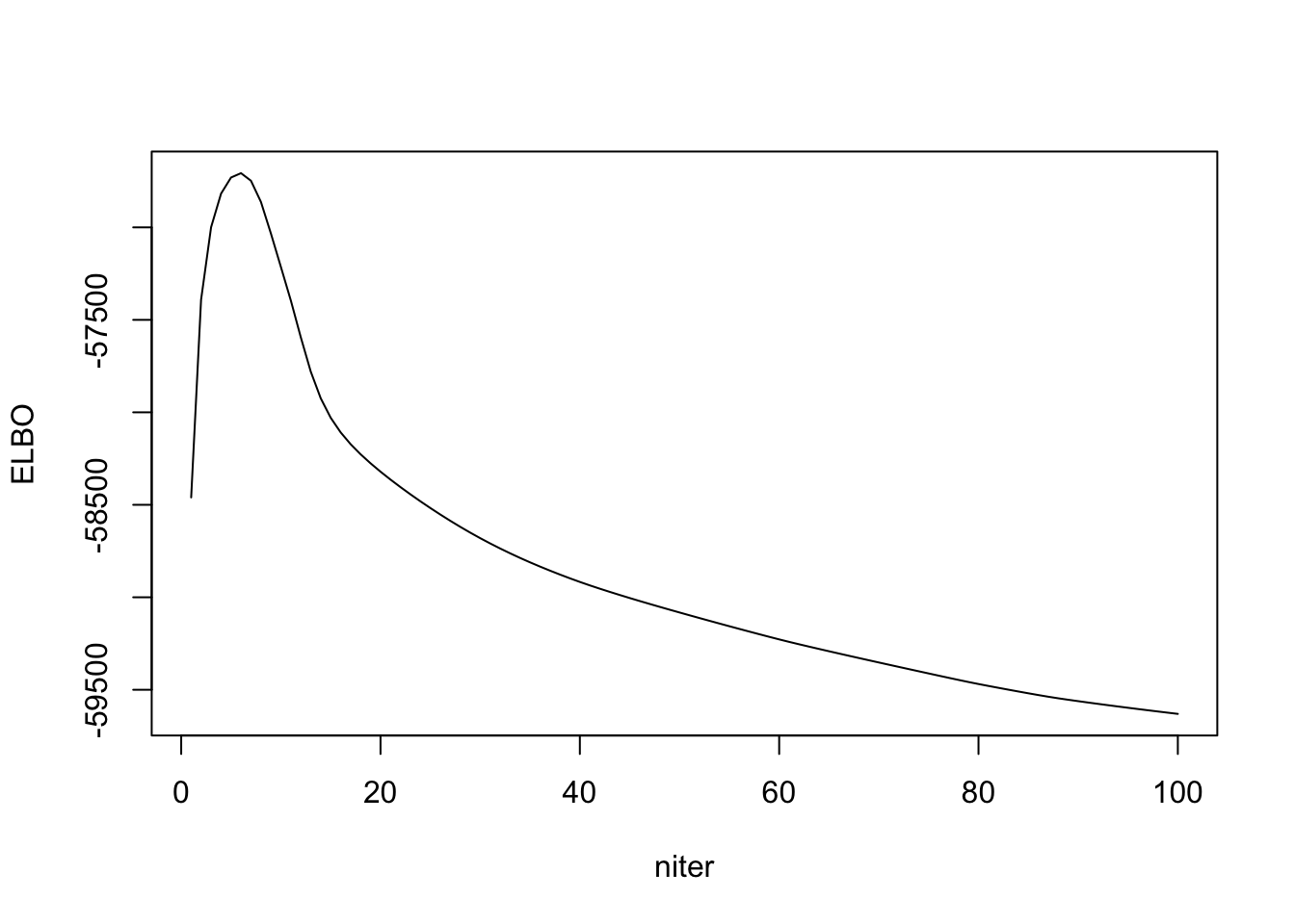

Version	Author	Date
244ee32	zihao12	2019-10-12

plot(out_ebpmf_exp$KL, type = "l", xlab = "niter", ylab = "KL")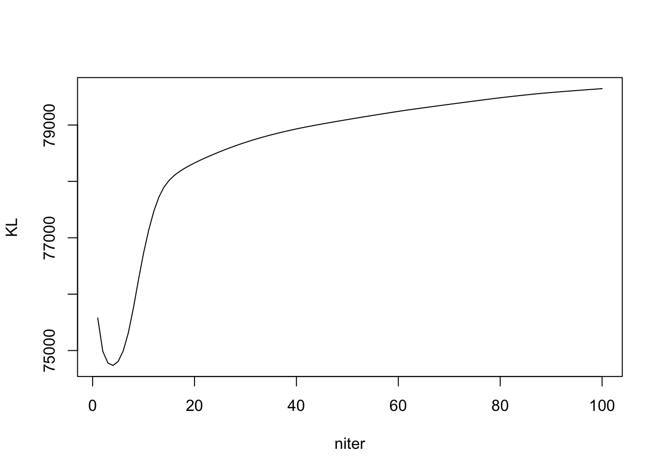

Version	Author	Date
244ee32	zihao12	2019-10-12

## experiment to see RMSE on Lambda
Lam_true = sim$L %*% t(sim$F)
try_experiment_rmse <- function(iter, Lam_true){
  test = ebpmf::ebpmf_point_gamma(sim$X, K, maxiter.out = iter)
  Lam = test$qg$qls_mean %*% t(test$qg$qfs_mean)
  return(sqrt(mean((Lam - Lam_true)^2)))
}

iters = seq(10,100,10)
rmses <- c()
for(iter in iters){
  rmse = try_experiment_rmse(iter, Lam_true)
  rmses = c(rmses, rmse)
}
rmses

 [1] 1.6422731 0.6258121 0.6182538 0.6162556 0.6150823 0.6142201 0.6133480
 [8] 0.6125504 0.6118396 0.6113208

plot(iters, rmses - min(rmses), main  = "distance to smallest rmse", xlab = "iter", type = "l")
points(iters, rmses - min(rmses))

Version	Author	Date
244ee32	zihao12	2019-10-12

Compare `ebpmf` and `nnmf`

simulation data

(The execution of the same code below is done in an interactive session in midway, and the result is shown below)

methods = c(); runtimes = c(); ll_trains = c(); ll_vals = c(); RMSEs = c()
## ebpmf_exponential_mixture
start = proc.time()
out = ebpmf::ebpmf_exponential_mixture(sim$X, K, m = 2, maxiter.out = 100)
runtime = proc.time() - start
lam_fit = out$qg$qls_mean %*% t(out$qg$qfs_mean)
ll_train = sum(dpois(sim$X, lambda = lam_fit, log = T))
ll_val   = sum(dpois(sim$Y, lambda = lam_fit, log = T))
RMSE     = mean((lam_fit - (sim$L %*% t(sim$F)))^2) 

methods = c(methods, "ebpmf_exponential_mixture")
runtimes = c(runtimes, runtime[[3]])
ll_trains = c(ll_trains, ll_train)
ll_vals   = c(ll_vals, ll_val)
RMSEs = c(RMSEs, RMSE)

## nnmf
W0 = out$qg$qls_mean
H0 = t(out$qg$qfs_mean)
start = proc.time()
out = NNLM::nnmf(sim$X, K,init = list(W0 = W0, H0 = H0), loss = "mkl", method = "lee", max.iter = 100, rel.tol = -1)
runtime = proc.time() - start
lam_fit = out$W %*% out$H
ll_train = sum(dpois(sim$X, lambda = lam_fit, log = T))
ll_val   = sum(dpois(sim$Y, lambda = lam_fit, log = T))
RMSE     = mean((lam_fit - (sim$L %*% t(sim$F)))^2) 

methods = c(methods, "NNMF")
runtimes = c(runtimes, runtime[[3]])
ll_trains = c(ll_trains, ll_train)
ll_vals   = c(ll_vals, ll_val)
RMSEs = c(RMSEs, RMSE)

## ebpmf_point_gamma
start = proc.time()
out = ebpmf::ebpmf_point_gamma(sim$X, K,maxiter.out = 100)
runtime = proc.time() - start
lam_fit = out$qg$qls_mean %*% t(out$qg$qfs_mean)
ll_train = sum(dpois(sim$X, lambda = lam_fit, log = T))
ll_val   = sum(dpois(sim$Y, lambda = lam_fit, log = T))
RMSE     = mean((lam_fit - (sim$L %*% t(sim$F)))^2) 
methods = c(methods, "ebpmf_point_gamma")
runtimes = c(runtimes, runtime[[3]])
ll_trains = c(ll_trains, ll_train)
ll_vals   = c(ll_vals, ll_val)
RMSEs = c(RMSEs, RMSE)

df <- data.frame(method = methods, runtime = runtimes, ll_train = ll_trains, ll_val = ll_vals, RMSE = RMSEs)

df = readRDS("output/Issue_ebpmf_issue2_df1.Rds")
df

                     method runtime  ll_train    ll_val      RMSE
1 ebpmf_exponential_mixture   6.014 -5812.834 -6011.257 0.3804012
2                      NNMF   0.135 -5652.354 -6150.184 0.6761194
3         ebpmf_point_gamma   8.778 -5810.426 -6023.255 0.3743813

real data

K = 2
maxiter.out = 100

(The execution of the same code below is done in an interactive session in midway, and the result is shown below)

methods = c(); runtimes = c(); ll_trains = c(); ll_vals = c(); 
## ebpmf_exponential_mixture
start = proc.time()
out = ebpmf::ebpmf_exponential_mixture(real$X, K, m = 2, maxiter.out = maxiter.out)
runtime = proc.time() - start
lam_fit = out$qg$qls_mean %*% t(out$qg$qfs_mean)
ll_train = sum(dpois(real$X, lambda = lam_fit, log = T))
ll_val   = sum(dpois(real$Y, lambda = lam_fit, log = T))

methods = c(methods, "ebpmf_exponential_mixture")
runtimes = c(runtimes, runtime[[3]])
ll_trains = c(ll_trains, ll_train)
ll_vals   = c(ll_vals, ll_val)

## nnmf
W0 = out$qg$qls_mean
H0 = t(out$qg$qfs_mean)
start = proc.time()
out = NNLM::nnmf(real$X, K,init = list(W0 = W0, H0 = H0), loss = "mkl", method = "lee", max.iter = maxiter.out, rel.tol = -1)
runtime = proc.time() - start
lam_fit = out$W %*% out$H
ll_train = sum(dpois(real$X, lambda = lam_fit, log = T))
ll_val   = sum(dpois(real$Y, lambda = lam_fit, log = T))

methods = c(methods, "NNMF")
runtimes = c(runtimes, runtime[[3]])
ll_trains = c(ll_trains, ll_train)
ll_vals   = c(ll_vals, ll_val)

## ebpmf_point_gamma
start = proc.time()
out = ebpmf::ebpmf_point_gamma(real$X, K,maxiter.out = maxiter.out)
runtime = proc.time() - start
lam_fit = out$qg$qls_mean %*% t(out$qg$qfs_mean)
ll_train = sum(dpois(real$X, lambda = lam_fit, log = T))
ll_val   = sum(dpois(real$Y, lambda = lam_fit, log = T))
methods = c(methods, "ebpmf_point_gamma")
runtimes = c(runtimes, runtime[[3]])
ll_trains = c(ll_trains, ll_train)
ll_vals   = c(ll_vals, ll_val)

df <- data.frame(method = methods, runtime = runtimes, ll_train = ll_trains, ll_val = ll_vals)

df = readRDS("output/Issue_ebpmf_issue2_df2.Rds")
df

                     method runtime  ll_train    ll_val
1 ebpmf_exponential_mixture 179.030 -976886.5 -984033.4
2                      NNMF  15.181 -962786.6 -974926.8
3         ebpmf_point_gamma 208.358 -977285.2 -984566.8

Comment

Our ebpmf methods do better in simulation data in validation, but much worse in real 10x-genomics dataset.

sessionInfo()

R version 3.5.1 (2018-07-02)
Platform: x86_64-apple-darwin15.6.0 (64-bit)
Running under: macOS  10.14

Matrix products: default
BLAS: /Library/Frameworks/R.framework/Versions/3.5/Resources/lib/libRblas.0.dylib
LAPACK: /Library/Frameworks/R.framework/Versions/3.5/Resources/lib/libRlapack.dylib

locale:
[1] en_US.UTF-8/en_US.UTF-8/en_US.UTF-8/C/en_US.UTF-8/en_US.UTF-8

attached base packages:
[1] stats     graphics  grDevices utils     datasets  methods   base     

other attached packages:
[1] NNLM_0.4.2   gtools_3.8.1 ebpmf_0.1.0 

loaded via a namespace (and not attached):
 [1] workflowr_1.4.0 Rcpp_1.0.2      digest_0.6.21   rprojroot_1.3-2
 [5] backports_1.1.5 git2r_0.25.2    magrittr_1.5    evaluate_0.14  
 [9] ebpm_0.0.0.9000 stringi_1.4.3   fs_1.3.1        whisker_0.3-2  
[13] rmarkdown_1.13  tools_3.5.1     stringr_1.4.0   glue_1.3.1     
[17] mixsqp_0.1-121  xfun_0.8        yaml_2.2.0      compiler_3.5.1 
[21] htmltools_0.3.6 knitr_1.25

Issue_ebpmf_issue2

zihao12

2019-10-12

Goal

dataset

ELBOs and RMSE

ELBO and KL

ebpmf_exponential_mixture

ebpmf_exponential_mixture

Compare ebpmf and nnmf

simulation data

real data

Comment

`ebpmf_exponential_mixture`

`ebpmf_exponential_mixture`

Compare `ebpmf` and `nnmf`