Compare_scd_lee

Goal

I find that fitting NMF model with lee and scd can get very different result.

Setup

Data generating model: here the mean structure is rank-1. \[ \begin{align} & \Lambda_{ij} = l f_j\\ & X_{ij} \sim Pois(\Lambda_{ij}) \end{align} \] ## Experiment I fit the data from above model with \(K = 2\). Ideally, we hope to get the \(l^1 \approx l, l^2 \approx 0\). But we can also get \(l^1 \approx cl, l^2 \approx (1-c)l\). We prefer the first one for our application.

sim_pois_rank1 <- function(n, p, seed = 123){
  set.seed(seed)
  L = matrix(replicate(n, 1), ncol = 1)
  F = matrix(sample(seq(1,1000,length.out = p)), ncol = 1)
  Lam = L %*% t(F)
  X = matrix(rpois(n*p, Lam), nrow = n)
  Y = matrix(rpois(n*p, Lam), nrow = n)
  ll_train = sum(dpois(X, Lam, log = T))
  ll_val = sum(dpois(Y, Lam, log = T))
  return(list(X = X, Y = Y, L = L, F = F, Lam = Lam, ll_train = ll_train, ll_val  = ll_val))
}


Ep_Z <- function(X, L, F){
  n = nrow(L)
  p = nrow(F)
  K = ncol(L)
  Z = array(dim = c(n, p, K))
  Lam = L %*% t(F)
  for(k in 1:K){
    lam_k = outer(L[,k], F[,k], "*")
    Z[,,k] = X * lam_k/Lam
  }
  return(Z)
}

# Scale each column of A so that the entries in each column sum to 1;
# i.e., colSums(scale.cols(A)) should return a vector of ones.
scale.cols <- function (A)
  apply(A,2,function (x) x/sum(x))

# Convert the parameters (factors & loadings) for the Poisson model to
# the factors and loadings for the multinomial model. The return value
# "s" gives the Poisson rates for generating the "document" sizes.
poisson2multinom <- function (F, L) {
  L <- t(t(L) * colSums(F))
  s <- rowSums(L)
  L <- L / s
  F <- scale.cols(F)
  return(list(F = F,L = L,s = s))
}

Simulate data

n = 50
p = 100
sim = sim_pois_rank1(n, p)

Fit with random initialization

Fit two models with \(K = 2\). Both are randomly initialized.

## lee
fit_lee = NNLM::nnmf(A = sim$X, k = 2, loss = "mkl", method = "lee", max.iter = 1000)
## scd
fit_scd = NNLM::nnmf(A = sim$X, k = 2, loss = "mkl", method = "scd", max.iter = 1000)

Below I show the two loadings from lee and scd. (I transform the L, F from Poisson model into multinomial model for better visual comparison)

p2m_res = poisson2multinom(F  = t(fit_scd$H), L = fit_scd$W)
L_df = data.frame(p2m_res$L)
colnames(L_df) = c("loading1", "loading2")
hist(L_df$loading1, col = "red", xlim=c(0, 1), xlab = "loading proportion", main = "scd")
hist(L_df$loading2, col = "blue", add = T)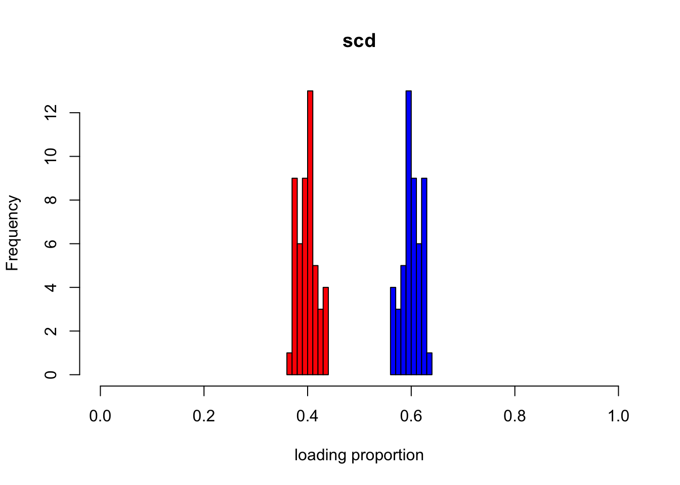

p2m_res = poisson2multinom(F  = t(fit_lee$H), L = fit_lee$W)
L_df = data.frame(p2m_res$L)
colnames(L_df) = c("loading1", "loading2")
hist(L_df$loading1, col = "red", xlim=c(0, 1), xlab = "loading proportion", main = "lee")
hist(L_df$loading2, col = "blue", add = T)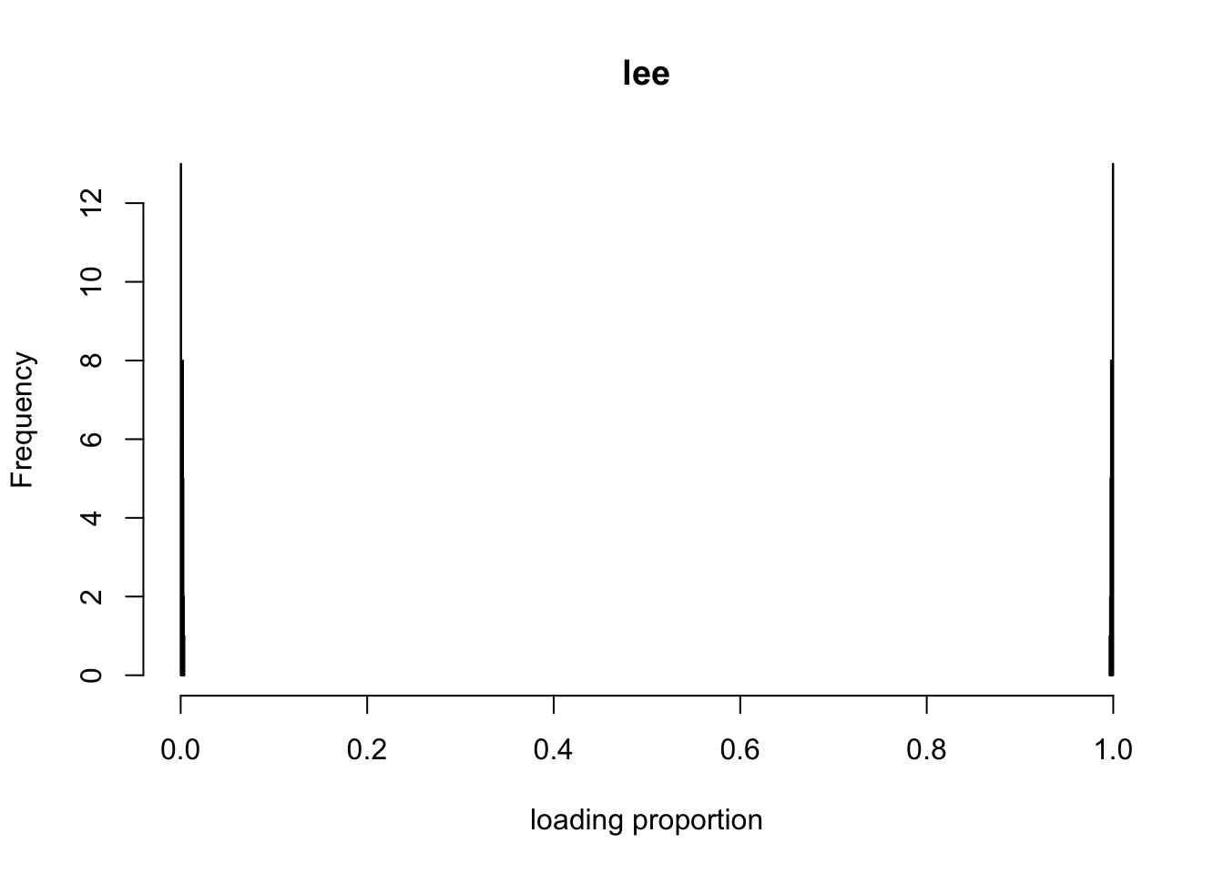

Fit with scd using initialization from lee.

fit_scd2 = NNLM::nnmf(A = sim$X, k = 2, init = list(W = fit_lee$W, H = fit_lee$H),loss = "mkl", method = "scd", max.iter = 1000)
p2m_res = poisson2multinom(F  = t(fit_scd2$H), L = fit_scd2$W)
L_df = data.frame(p2m_res$L)
colnames(L_df) = c("loading1", "loading2")
hist(L_df$loading1, col = "red", xlim=c(0, 1), xlab = "loading proportion", main = "scd initialized from lee")
hist(L_df$loading2, col = "blue", add = T)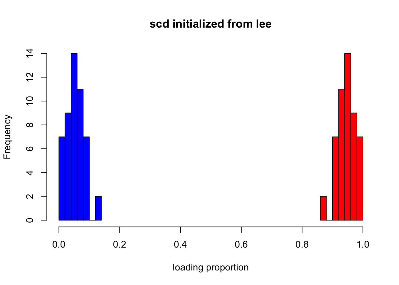

It gets much better, but still scd tends to make the two components closer to each other.

Finally lets’ show the rmse and loglikelihood from the fits

compute_rmse <- function(lam, fit){
  Lam_fit = fit$W %*% fit$H
  return(sqrt(mean((sim$Lam - Lam_fit)^2)))
}

compute_ll <- function(X, fit){
  Lam = fit$W %*% fit$H
  return(sum(dpois(X, Lam, log = T)))
}

## RMSE
data.frame(lee = compute_rmse(sim$Lam, fit_lee),
           scd = compute_rmse(sim$Lam, fit_scd),
           scd_from_lee = compute_rmse(sim$Lam, fit_scd2))

       lee      scd scd_from_lee
1 4.470766 6.440674     6.917587

## Loglikelihood (Training)
data.frame(lee = compute_ll(sim$X, fit_lee),
           scd = compute_ll(sim$X, fit_scd),
           scd_from_lee = compute_ll(sim$X, fit_scd2))

        lee       scd scd_from_lee
1 -21615.08 -21538.96    -21527.44

## Loglikelihood (Validation)
data.frame(lee = compute_ll(sim$Y, fit_lee),
           scd = compute_ll(sim$Y, fit_scd),
           scd_from_lee = compute_ll(sim$Y, fit_scd2))

        lee    scd scd_from_lee
1 -21871.25 -21933    -21947.02

Session information

sessionInfo()

R version 3.5.1 (2018-07-02)
Platform: x86_64-apple-darwin15.6.0 (64-bit)
Running under: macOS  10.14

Matrix products: default
BLAS: /Library/Frameworks/R.framework/Versions/3.5/Resources/lib/libRblas.0.dylib
LAPACK: /Library/Frameworks/R.framework/Versions/3.5/Resources/lib/libRlapack.dylib

locale:
[1] en_US.UTF-8/en_US.UTF-8/en_US.UTF-8/C/en_US.UTF-8/en_US.UTF-8

attached base packages:
[1] stats     graphics  grDevices utils     datasets  methods   base     

other attached packages:
[1] NNLM_0.4.2

loaded via a namespace (and not attached):
 [1] workflowr_1.4.0 Rcpp_1.0.2      digest_0.6.22   rprojroot_1.3-2
 [5] backports_1.1.5 git2r_0.25.2    magrittr_1.5    evaluate_0.14  
 [9] stringi_1.4.3   fs_1.3.1        whisker_0.3-2   rmarkdown_1.13 
[13] tools_3.5.1     stringr_1.4.0   glue_1.3.1      xfun_0.8       
[17] yaml_2.2.0      compiler_3.5.1  htmltools_0.3.6 knitr_1.25