Compare_ebpm_vs_ash_pois
zihao12
2019-09-28
Last updated: 2019-09-30
Checks: 7 0
Knit directory: ebpmf_demo/
This reproducible R Markdown analysis was created with workflowr (version 1.4.0). The Checks tab describes the reproducibility checks that were applied when the results were created. The Past versions tab lists the development history.
Great! Since the R Markdown file has been committed to the Git repository, you know the exact version of the code that produced these results.
Great job! The global environment was empty. Objects defined in the global environment can affect the analysis in your R Markdown file in unknown ways. For reproduciblity it’s best to always run the code in an empty environment.
The command set.seed(20190923) was run prior to running the code in the R Markdown file. Setting a seed ensures that any results that rely on randomness, e.g. subsampling or permutations, are reproducible.
Great job! Recording the operating system, R version, and package versions is critical for reproducibility.
Nice! There were no cached chunks for this analysis, so you can be confident that you successfully produced the results during this run.
Great job! Using relative paths to the files within your workflowr project makes it easier to run your code on other machines.
Great! You are using Git for version control. Tracking code development and connecting the code version to the results is critical for reproducibility. The version displayed above was the version of the Git repository at the time these results were generated.
Note that you need to be careful to ensure that all relevant files for the analysis have been committed to Git prior to generating the results (you can use wflow_publish or wflow_git_commit). workflowr only checks the R Markdown file, but you know if there are other scripts or data files that it depends on. Below is the status of the Git repository when the results were generated:
Ignored files:
    Ignored:    .Rhistory
    Ignored:    .Rproj.user/

Untracked files:
    Untracked:  analysis/ebpmf_demo.Rmd
    Untracked:  docs/figure/test.Rmd/

Unstaged changes:
    Modified:   analysis/index.Rmd
Note that any generated files, e.g. HTML, png, CSS, etc., are not included in this status report because it is ok for generated content to have uncommitted changes.
These are the previous versions of the R Markdown and HTML files. If you’ve configured a remote Git repository (see ?wflow_git_remote), click on the hyperlinks in the table below to view them.
| File | Version | Author | Date | Message |
|---|---|---|---|---|
| html | 3dd3e5c | zihao12 | 2019-09-30 | Build site. |
| Rmd | 2c4ab46 | zihao12 | 2019-09-30 | update demo after library changes |
| html | f73f934 | zihao12 | 2019-09-30 | Build site. |
| Rmd | 3ee50d3 | zihao12 | 2019-09-30 | add more explanation |
| html | 5cec335 | zihao12 | 2019-09-28 | Build site. |
| html | c966a85 | zihao12 | 2019-09-28 | Build site. |
| Rmd | 255ebde | zihao12 | 2019-09-28 | Compare ebpm vs ash_pois |
Compare ebpm_exponential_mixture vs ash_pois
I use ebpm from https://github.com/stephenslab/ebpm, (branch “zihao”) and ash_pois from https://github.com/stephens999/ashr/blob/master/R/ash_pois.R
Experiment setup
I simulate \(x_i \sim pois(s_i \lambda_i), \lambda_i \sim \sum_k^{K} \pi_k exp(b_k), \forall i = 1 ,..., 4000\) with \(K = 50\). I use \(s_i = 1\).
Then I fit ash_pois and ebpm_exponential_mixture on given \(x, s\)s
library(gtools)
library(ebpm)
library(ashr)
library(ggplot2)
Warning: package 'ggplot2' was built under R version 3.5.2library(mixsqp)
n = 4000
d = 50sim_mgamma <- function(a,b,pi){
idx = which(rmultinom(1,1,pi) == 1)
return(rgamma(1, shape = a[idx], rate = b[idx]))
}
## simulate a poisson mean problem
simulate_pm <- function(n, d, seed = 123){
set.seed(seed)
## simulate grid
a = replicate(d,1)
b = 10*runif(d)
grid = list(a = a, b = b)
pi <- rdirichlet(1,rep(1/d, d))
lam_true = replicate(n, sim_mgamma(a,b,pi))
s = replicate(length(lam_true), 1)
#s = 2*runif(length(lam_true))
x = rpois(length(lam_true),s*lam_true)
ll_lam = sum(dpois(x, s*lam_true, log = T))
return(list(x = x, s = s, lam_true = lam_true, pi = pi, grid = grid))
}
rmse <- function(x,y){
return(sqrt(mean((x-y)^2)))
}sim = simulate_pm(n = n, d = d)
start = proc.time()
out_ebpm_exponential_mixture = ebpm::ebpm_exponential_mixture(sim$x, s = sim$s, m = 1.1)
out_ebpm_exponential_mixture[["runtime"]] = (proc.time() - start)[[3]]
start = proc.time()
out_ash = ash_pois(sim$x, scale = sim$s, link = "identity")
out_ash[["runtime"]] = (proc.time() - start)[[3]]
print(sprintf("runtime for ebpm_exponential_mixture: %f", out_ebpm_exponential_mixture$runtime))[1] "runtime for ebpm_exponential_mixture: 0.195000"print(sprintf("runtime for ash_pois : %f", out_ash$runtime))[1] "runtime for ash_pois : 3.184000"compare RMSE against \(\lambda_{true}\)
df = data.frame(n = 1:length(sim$x), x = sim$x, s =  sim$s, lam_true = sim$lam_true,
                lam_hat_ebpm_exponential_mixture = out_ebpm_exponential_mixture$posterior$mean,
                lam_hat_ash_pois = out_ash$result[["PosteriorMean"]])

print(sprintf("rmse(lam_ash_pois, lam_true)                     = %f", rmse(df$lam_true, df$lam_hat_ash_pois)))
[1] "rmse(lam_ash_pois, lam_true) = 0.122928"print(sprintf("rmse(lam_hat_ebpm_exponential_mixture, lam_true) = %f", rmse(df$lam_true, df$lam_hat_ebpm_exponential_mixture)))[1] "rmse(lam_hat_ebpm_exponential_mixture, lam_true) = 0.122431"visualize poasterior means
ggplot(df) +
  geom_point(aes(x = lam_hat_ash_pois, y = lam_hat_ebpm_exponential_mixture), color = "blue") +
  labs(x = "lam_hat_ash_pois", y = "lam_hat_ebpm_exponential_mixture")+
  geom_abline(slope = 1, intercept = 0)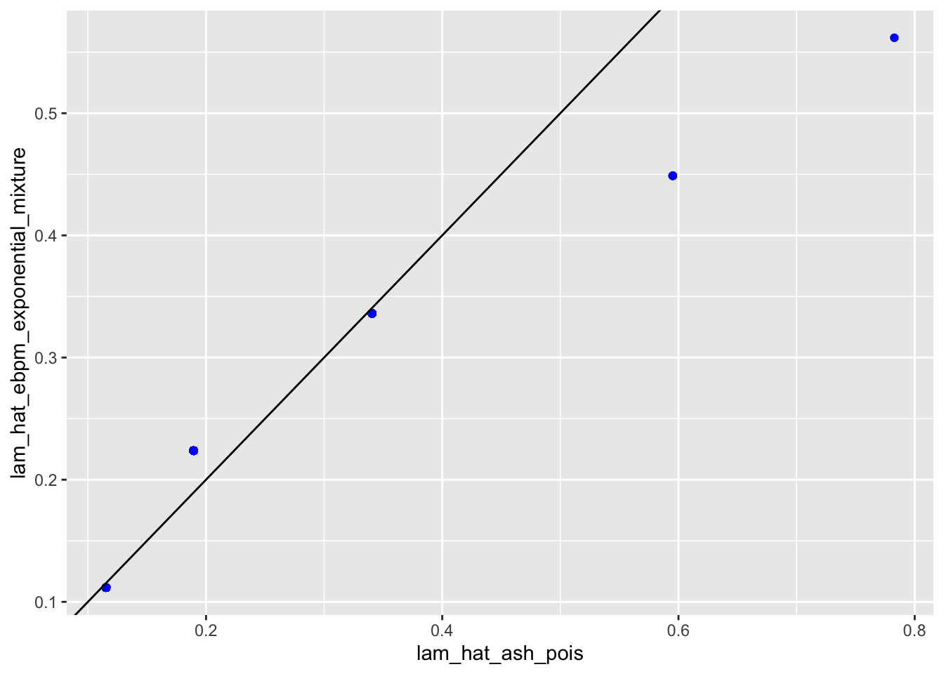
Below I sort \(x\) and plot \(\lambda\)s against the sorting index. Expecting to see horizontal lines (\(x\) takes value in integers,and for fixed \(x\), the posterior mean is fixed).
df_sort = df[order(df$x),]
df_sort$n = 1:length(sim$x)

ggplot(df_sort) +
  geom_point(aes(x = n, y = lam_true, color = "true"), cex = 0.5) +
    labs(x = "index", y = "lam", title = "ash_pois vs ebpm_exponential_mixture") +
  geom_point(aes(x = n, y = lam_hat_ebpm_exponential_mixture, color = "ebpm_exponential_mixture"), cex = 0.5) +
  geom_point(aes(x = n, y = lam_hat_ash_pois, color = "ash"), cex = 0.5) +
  guides(fill = "color")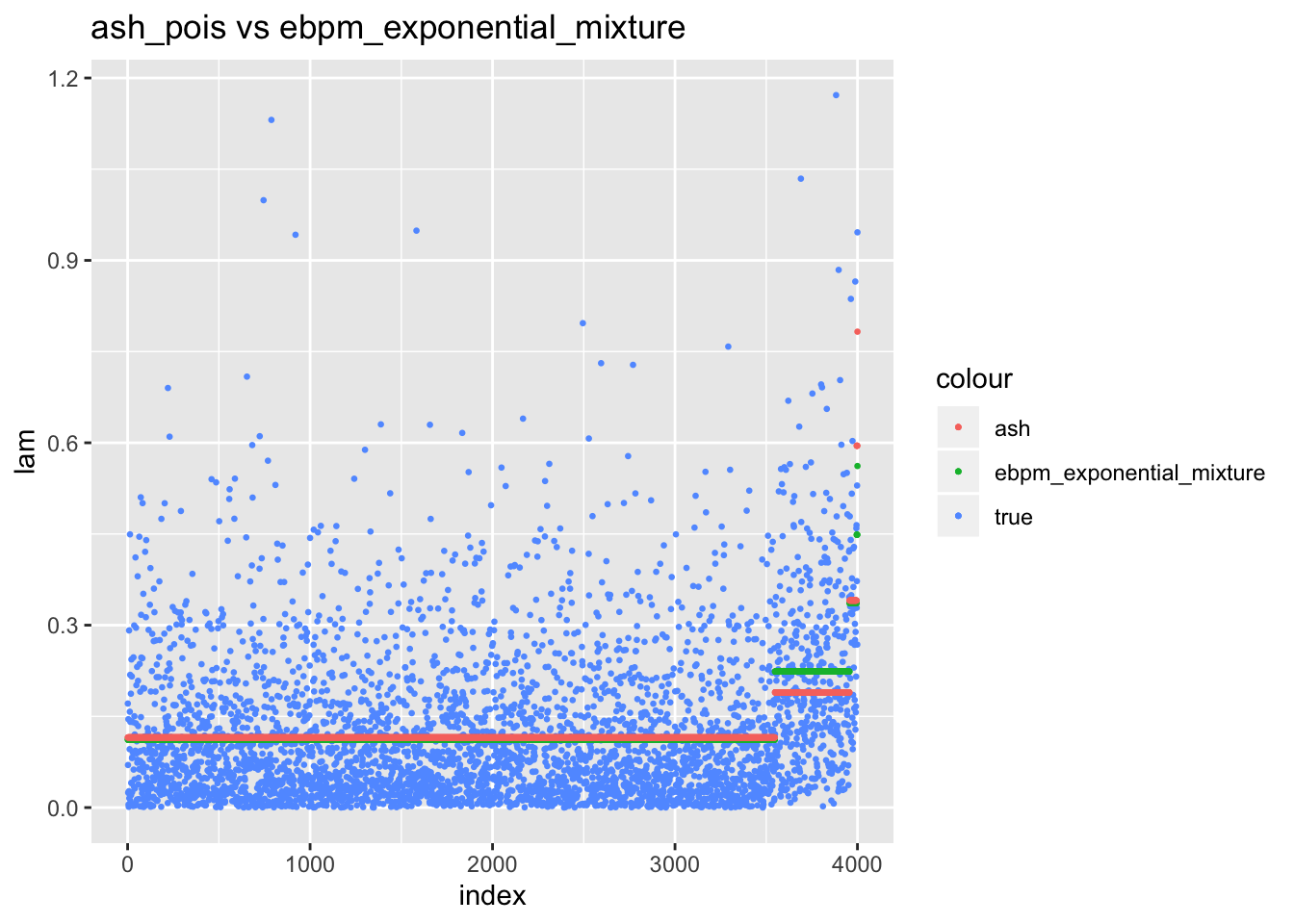
sessionInfo()R version 3.5.1 (2018-07-02)
Platform: x86_64-apple-darwin15.6.0 (64-bit)
Running under: macOS 10.14
Matrix products: default
BLAS: /Library/Frameworks/R.framework/Versions/3.5/Resources/lib/libRblas.0.dylib
LAPACK: /Library/Frameworks/R.framework/Versions/3.5/Resources/lib/libRlapack.dylib
locale:
[1] en_US.UTF-8/en_US.UTF-8/en_US.UTF-8/C/en_US.UTF-8/en_US.UTF-8
attached base packages:
[1] stats graphics grDevices utils datasets methods base
other attached packages:
[1] mixsqp_0.1-120 ggplot2_3.2.1 ashr_2.2-38 ebpm_0.0.0.9000
[5] gtools_3.8.1
loaded via a namespace (and not attached):
[1] Rcpp_1.0.2 pillar_1.4.2 compiler_3.5.1
[4] git2r_0.25.2 workflowr_1.4.0 iterators_1.0.12
[7] tools_3.5.1 digest_0.6.21 evaluate_0.14
[10] tibble_2.1.3 gtable_0.3.0 lattice_0.20-38
[13] pkgconfig_2.0.3 rlang_0.4.0 Matrix_1.2-17
[16] foreach_1.4.7 yaml_2.2.0 parallel_3.5.1
[19] xfun_0.8 withr_2.1.2 dplyr_0.8.1
[22] stringr_1.4.0 knitr_1.25 fs_1.3.1
[25] tidyselect_0.2.5 rprojroot_1.3-2 grid_3.5.1
[28] glue_1.3.1 R6_2.4.0 rmarkdown_1.13
[31] purrr_0.3.2 magrittr_1.5 whisker_0.3-2
[34] backports_1.1.4 scales_1.0.0 codetools_0.2-16
[37] htmltools_0.3.6 MASS_7.3-51.4 assertthat_0.2.1
[40] colorspace_1.4-1 labeling_0.3 stringi_1.4.3
[43] lazyeval_0.2.2 doParallel_1.0.15 pscl_1.5.2
[46] munsell_0.5.0 truncnorm_1.0-8 SQUAREM_2017.10-1
[49] crayon_1.3.4