kos_K100_ebpmf.alpha_v0.3.9
zihao12
2020-05-11
Last updated: 2020-05-18
Checks: 7 0
Knit directory: ebpmf_data_analysis/
This reproducible R Markdown analysis was created with workflowr (version 1.6.2). The Checks tab describes the reproducibility checks that were applied when the results were created. The Past versions tab lists the development history.
Great! Since the R Markdown file has been committed to the Git repository, you know the exact version of the code that produced these results.
Great job! The global environment was empty. Objects defined in the global environment can affect the analysis in your R Markdown file in unknown ways. For reproduciblity it’s best to always run the code in an empty environment.
The command set.seed(20200511) was run prior to running the code in the R Markdown file. Setting a seed ensures that any results that rely on randomness, e.g. subsampling or permutations, are reproducible.
Great job! Recording the operating system, R version, and package versions is critical for reproducibility.
Nice! There were no cached chunks for this analysis, so you can be confident that you successfully produced the results during this run.
Great job! Using relative paths to the files within your workflowr project makes it easier to run your code on other machines.
Great! You are using Git for version control. Tracking code development and connecting the code version to the results is critical for reproducibility.
The results in this page were generated with repository version 17d7f38. See the Past versions tab to see a history of the changes made to the R Markdown and HTML files.
Note that you need to be careful to ensure that all relevant files for the analysis have been committed to Git prior to generating the results (you can use wflow_publish or wflow_git_commit). workflowr only checks the R Markdown file, but you know if there are other scripts or data files that it depends on. Below is the status of the Git repository when the results were generated:
Ignored files:
    Ignored:    .Rhistory
    Ignored:    .Rproj.user/
    Ignored:    analysis/ebpmf_bg_tutorial_cache/

Untracked files:
    Untracked:  analysis/compare_LF.R
    Untracked:  analysis/plot_topic_words.R
    Untracked:  code/.util.R.swp
Note that any generated files, e.g. HTML, png, CSS, etc., are not included in this status report because it is ok for generated content to have uncommitted changes.
These are the previous versions of the repository in which changes were made to the R Markdown (analysis/kos_K100_ebpmf.alpha_v0.3.9.Rmd) and HTML (docs/kos_K100_ebpmf.alpha_v0.3.9.html) files. If you’ve configured a remote Git repository (see ?wflow_git_remote), click on the hyperlinks in the table below to view the files as they were in that past version.
| File | Version | Author | Date | Message |
|---|---|---|---|---|
| Rmd | 17d7f38 | zihao12 | 2020-05-18 | update analysis for v0.3.9 |
| html | 88cc049 | zihao12 | 2020-05-16 | Build site. |
| Rmd | 20a60fd | zihao12 | 2020-05-16 | update analysis for results in v0.3.9 |
| html | 7928026 | zihao12 | 2020-05-16 | Build site. |
| Rmd | 3e38a38 | zihao12 | 2020-05-16 | analysis for results in v0.3.9 |
Introduction
- I apply
ebpmf.alpha(version 0.3.9) to KOS dataset. I use \(K = 100\). The data has \(n = 3430,p = 6906\) and sparsity around \(98\) percent.
- Besides, I also apply to
PMF(lee’s, but I implemented a version for sparse data) to the same dataset with the same initialization. In each iteration,ebpmf_bgdoes two things: MLE for prior and updates posterior. The second part has almost the same computation as inPMF.
model
\[\begin{align} & X_{ij} = \sum_k Z_{ijk}\\ & Z_{ijk} \sim Pois(l_{i0} f_{j0} l_{ik} f_{jk})\\ & l_{ik} \sim g_{L, k}(.), f_{jk} \sim g_{F, k}(.) \end{align}\]For details see ebpmf_bg
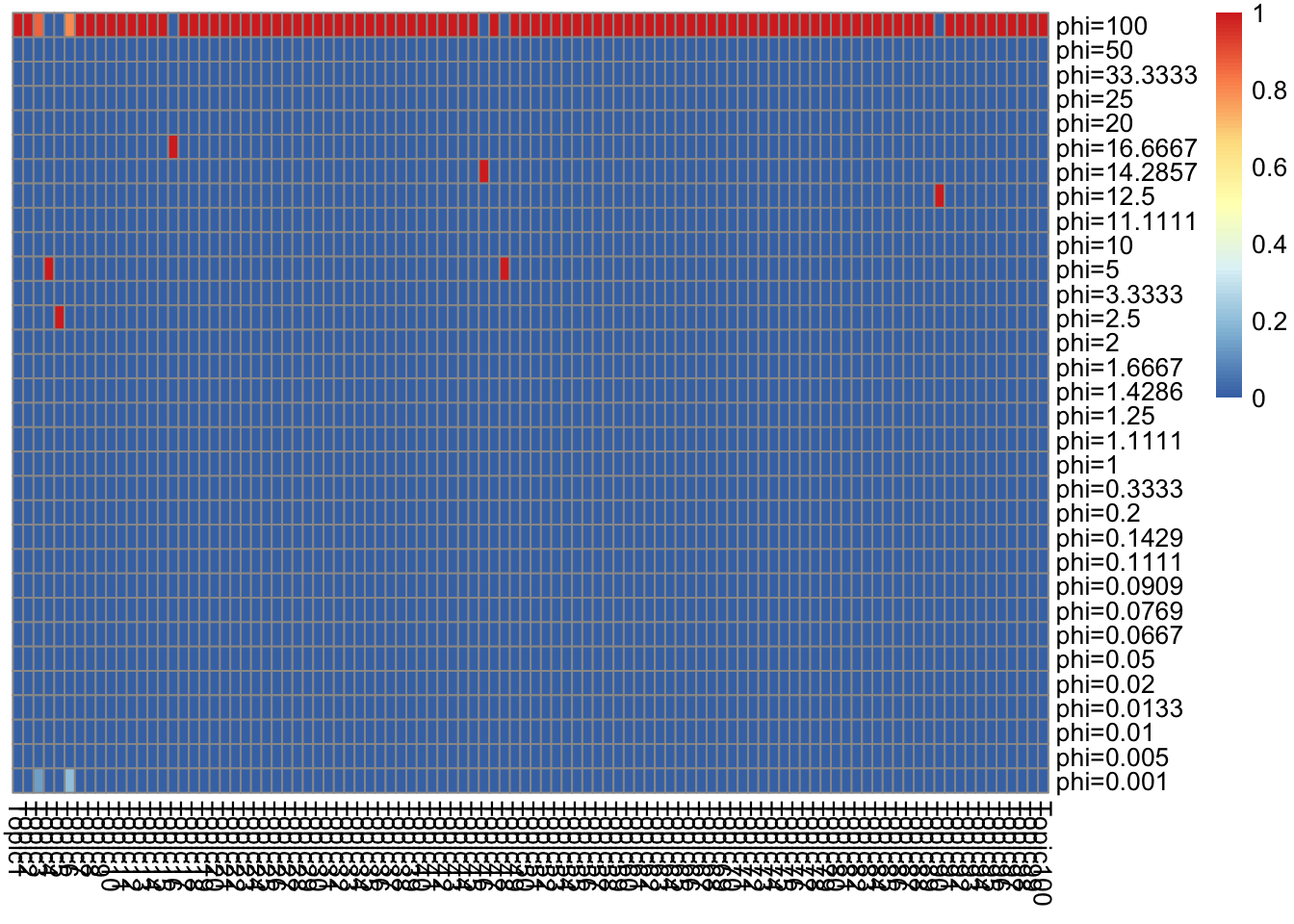
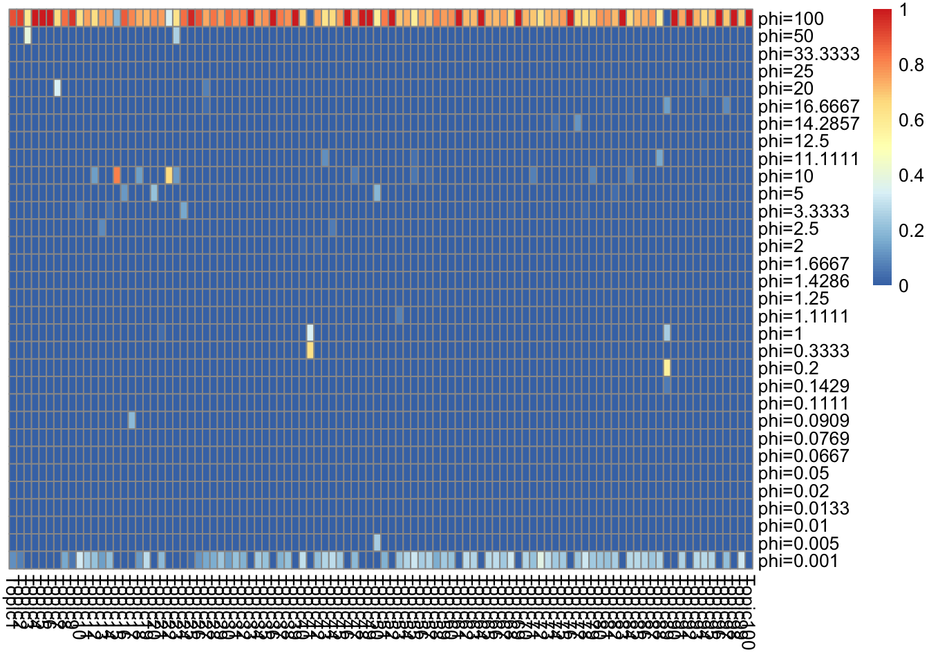
prior options
I use gamma mixture \(\sum_l \pi_{l} Ga(1/\phi_l, 1/\phi_l)\) as prior for both \(L, F\). Note that each grid component has \(E = 1, Var = \phi_L\)
initialization
I initialized with 50 runs of NNLM::nnmf (scd). Then I used medians of each row of \(L, F\) as \(l_{i0}, f_{j0}\), and \(l_{ik} = l^0_{ik}/l_{i0}, f_{jk} = f^0_{jk}/f_{j0}\).
library(pheatmap)Warning: package 'pheatmap' was built under R version 3.5.2library(gridExtra)
source("code/misc.R")
source("code/util.R")
output_dir = "output/uci_BoW/v0.3.9/"
data_dir = "data/uci_BoW/"
model_name = "kos_ebpmf_bg_initLF50_K100_maxiter2000.Rds"
model_pmf_name = "kos_pmf_initLF50_K100_maxiter2000.Rds"
dict_name = "vocab.kos.txt"
data_name = "docword.kos.txt"
Y = read_uci_bag_of_words(file= sprintf("%s/%s",
data_dir,data_name))
model = readRDS(sprintf("%s/%s", output_dir, model_name))
model_pmf = readRDS(sprintf("%s/%s", output_dir, model_pmf_name))
dict = read.csv(sprintf("%s/%s", data_dir, dict_name), header = FALSE)[,1]
dict = as.vector(dict)
K = ncol(model_pmf$L)
L_pmf = model_pmf$L; F_pmf = model_pmf$F
L_bg = model$l0 * model$qg$qls_mean; F_bg = model$f0 * model$qg$qfs_mean
lf = poisson2multinom(L=L_bg,F=F_bg)
lf_pmf = poisson2multinom(L = L_pmf,F = F_pmf)ELBO and runtime
plot(model$ELBO, xlab = "niter", ylab = "elbo")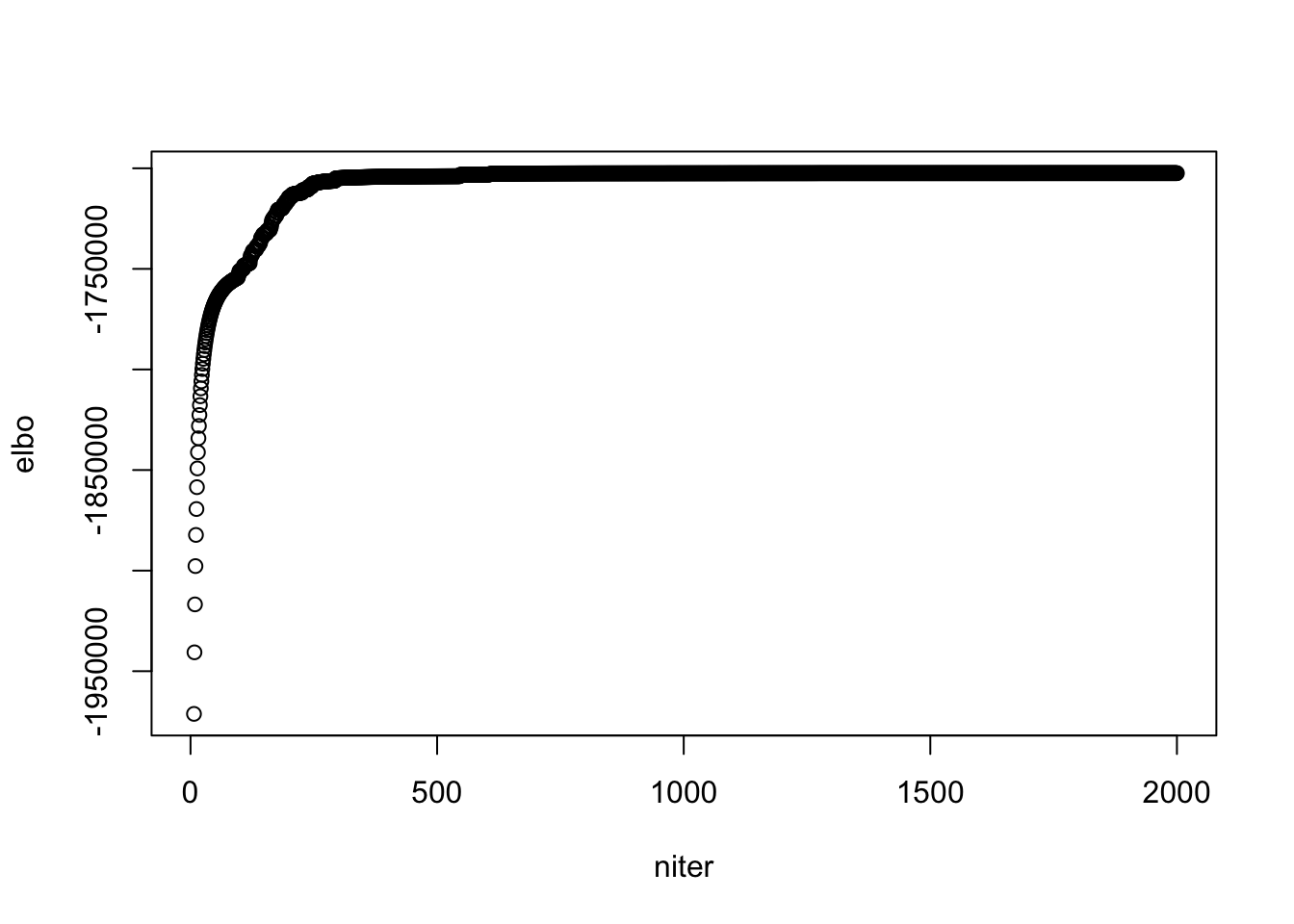
| Version | Author | Date |
|---|---|---|
| 7928026 | zihao12 | 2020-05-16 |
## see when it "converges"
plot(model$ELBO[1:400], xlab = "niter", ylab = "elbo")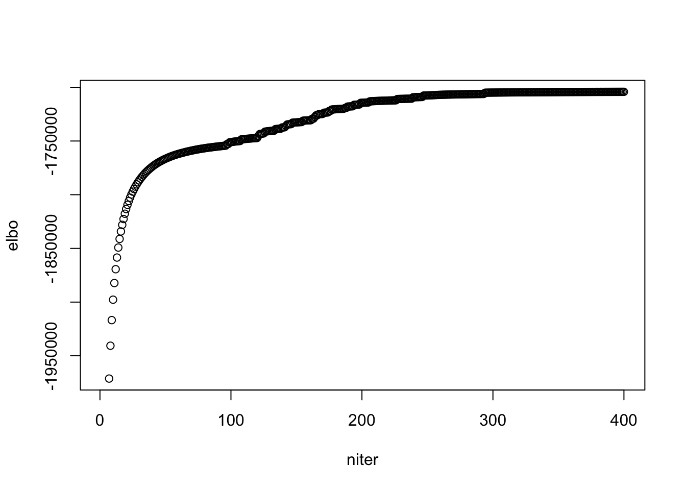
| Version | Author | Date |
|---|---|---|
| 7928026 | zihao12 | 2020-05-16 |
## ebpmf_bg runtime per iteration
model$runtime/length(model$ELBO)
user system elapsed
49.1382770 0.1047385 49.2636325 ## pmf runtime per iteration
model_pmf$runtime/length(model_pmf$log_liks) user system elapsed
23.3493840 0.0607845 23.4182915 look at priors in ebpmf_bg
look at \(s_k\) (ebpmf_bg)
\(s_k := \sum_i l_i0 \bar{l}_{ik}\). I make \(\sum_j f_{j0} = 1\) for interpretability.
d = sum(model$f0)
s_k = colSums(d * model$l0 * model$qg$qls_mean)
names(s_k) <- paste("Topic", 1:K, sep = "")
step = 5
for(i in 1:round(K/step)){
  print(round(s_k[((i-1)*step + 1):(i*step)]))
}
Topic1 Topic2 Topic3 Topic4 Topic5
6127 7488 2660 10167 9964
Topic6 Topic7 Topic8 Topic9 Topic10
2557 5557 11819 7535 5104
Topic11 Topic12 Topic13 Topic14 Topic15
5593 4821 7736 10043 4349
Topic16 Topic17 Topic18 Topic19 Topic20
7005 11345 10087 4514 5787
Topic21 Topic22 Topic23 Topic24 Topic25
6912 2635 7217 7775 8093
Topic26 Topic27 Topic28 Topic29 Topic30
14903 11400 8410 8391 5961
Topic31 Topic32 Topic33 Topic34 Topic35
7411 5711 9417 7548 7218
Topic36 Topic37 Topic38 Topic39 Topic40
7842 6813 5983 4770 6656
Topic41 Topic42 Topic43 Topic44 Topic45
2891 6891 8804 4176 6551
Topic46 Topic47 Topic48 Topic49 Topic50
6388 6488 7657 5764 4718
Topic51 Topic52 Topic53 Topic54 Topic55
6954 6695 6268 9018 5088
Topic56 Topic57 Topic58 Topic59 Topic60
6855 10080 5850 5235 4496
Topic61 Topic62 Topic63 Topic64 Topic65
7053 6959 7270 5365 5534
Topic66 Topic67 Topic68 Topic69 Topic70
7140 6980 8090 6387 4757
Topic71 Topic72 Topic73 Topic74 Topic75
12123 3861 7261 13980 5848
Topic76 Topic77 Topic78 Topic79 Topic80
4076 11736 6507 10753 9073
Topic81 Topic82 Topic83 Topic84 Topic85
11450 14064 5522 5565 7209
Topic86 Topic87 Topic88 Topic89 Topic90
9514 7169 7494 4002 5618
Topic91 Topic92 Topic93 Topic94 Topic95
9744 9667 6735 9001 6662
Topic96 Topic97 Topic98 Topic99 Topic100
5313 14731 6857 7350 6482 what does background capture
compared to rank-1 fit
Is the background very different from the rank-1 model? The rank-1 MLE has \(l_{i0} \propto \sum_j X_{ij}\) and \(f_{j0} \propto \sum_i X_{ij}\). Let’s see if the fitted background model is close to it.
Y_cs = Matrix::colSums(Y)
Y_cs_scaled = Y_cs/sum(Y_cs)
f0_scaled = model$f0/sum(model$f0)
plot(f0_scaled, Y_cs_scaled)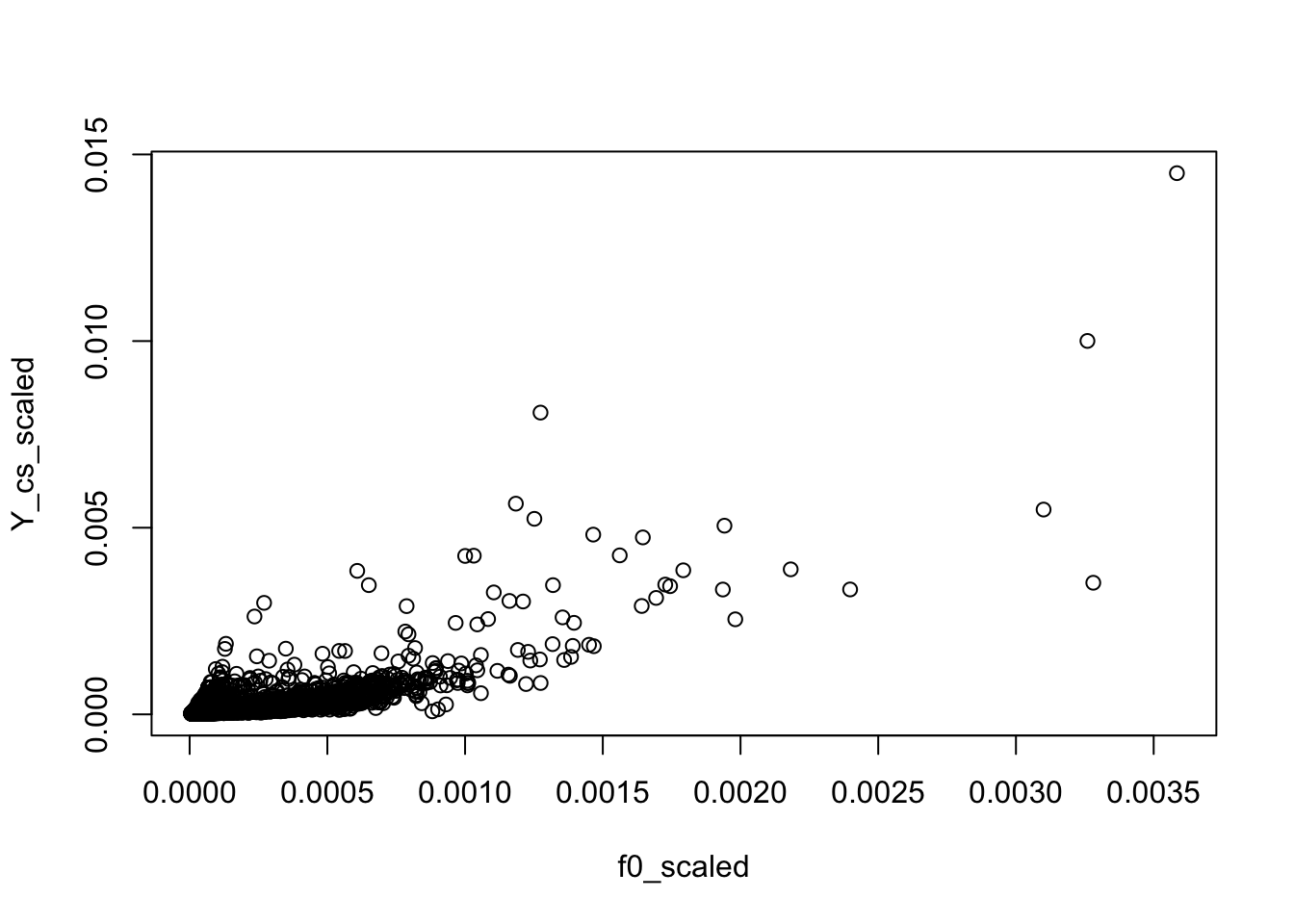
Y_rs = Matrix::rowSums(Y)
Y_rs_scaled = Y_rs/sum(Y_rs)
l0_scaled = model$l0/sum(model$l0)
plot(l0_scaled, Y_rs_scaled)
compared to median/mean of PMF fit
The median of L_pmf are all 0, so I use mean instead
f0_pmf = apply(F_pmf, 1, median)
f0_pmf_scaled = f0_pmf/sum(f0_pmf)

l0_pmf = apply(L_pmf, 1, mean)
l0_pmf_scaled = l0_pmf/sum(l0_pmf)

plot(f0_scaled, f0_pmf_scaled)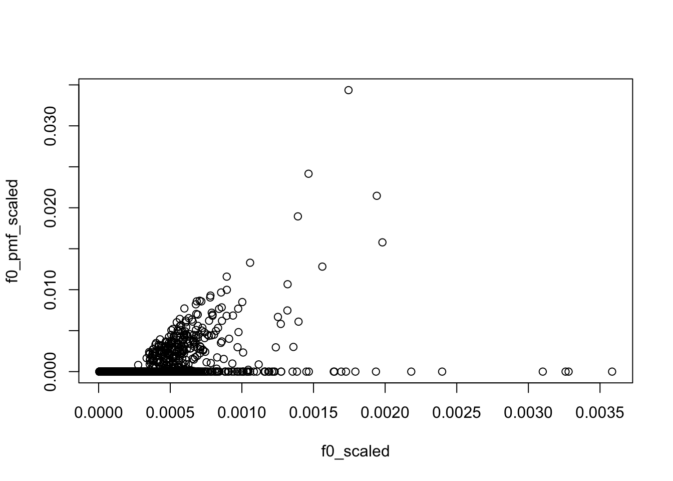
plot(l0_scaled, l0_pmf_scaled)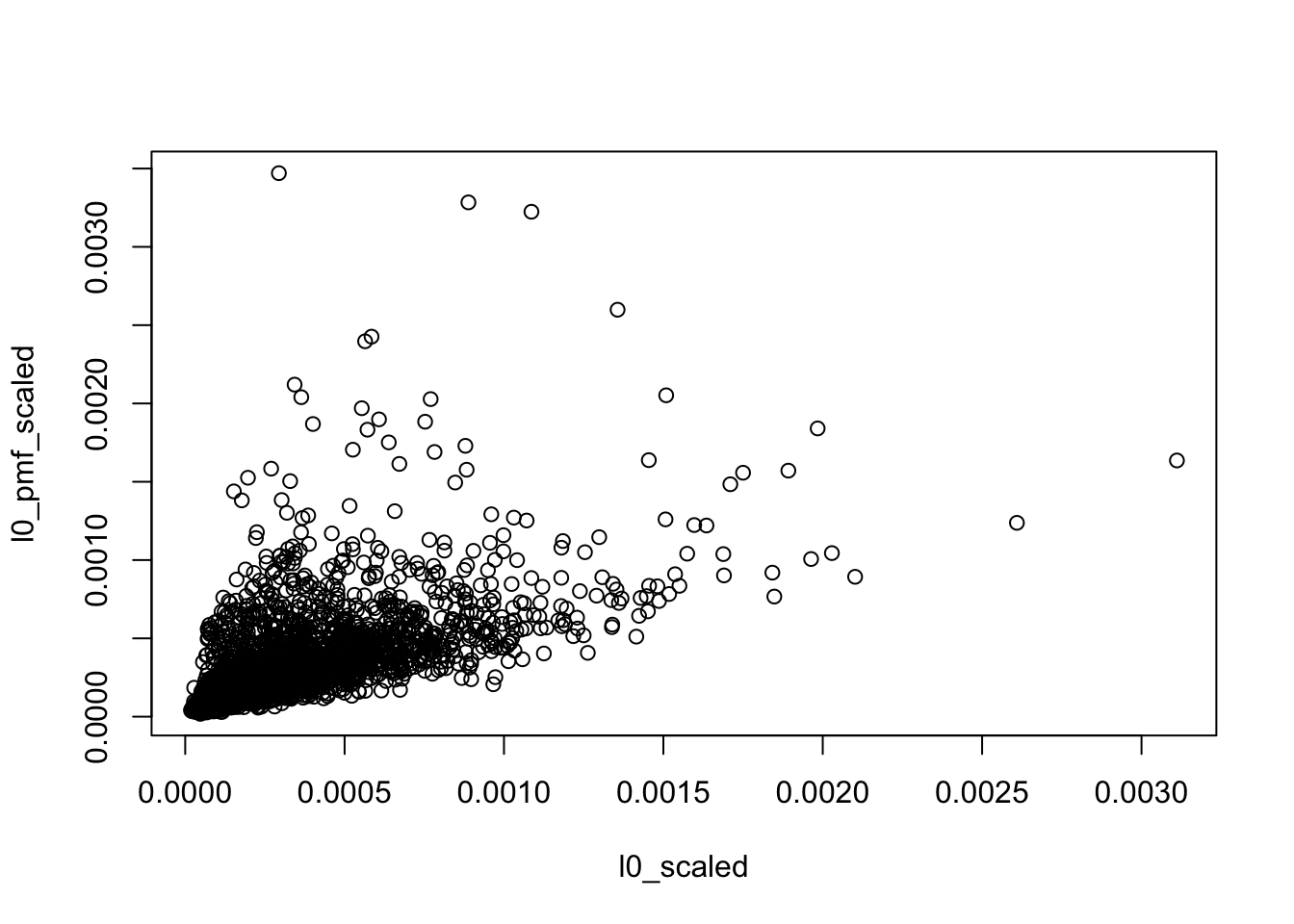
Compare \(L, F\) (in the context of PMF model)
See plots.
Note: I scale them as below
## scale L, F so that colSums(F) = 1
L_pmf = L_pmf %*% diag(colSums(F_pmf))
F_pmf = F_pmf %*% diag(1/colSums(F_pmf))

L_bg = L_bg %*% diag(colSums(F_bg))
F_bg = F_bg %*% diag(1/colSums(F_bg))
look at top words for topics
See plots
sessionInfo()R version 3.5.1 (2018-07-02)
Platform: x86_64-apple-darwin15.6.0 (64-bit)
Running under: macOS 10.14
Matrix products: default
BLAS: /Library/Frameworks/R.framework/Versions/3.5/Resources/lib/libRblas.0.dylib
LAPACK: /Library/Frameworks/R.framework/Versions/3.5/Resources/lib/libRlapack.dylib
locale:
[1] en_US.UTF-8/en_US.UTF-8/en_US.UTF-8/C/en_US.UTF-8/en_US.UTF-8
attached base packages:
[1] stats graphics grDevices utils datasets methods base
other attached packages:
[1] gridExtra_2.3 pheatmap_1.0.12
loaded via a namespace (and not attached):
[1] Rcpp_1.0.2 knitr_1.28 whisker_0.3-2 magrittr_1.5
[5] workflowr_1.6.2 munsell_0.5.0 lattice_0.20-38 colorspace_1.4-1
[9] R6_2.4.0 stringr_1.4.0 tools_3.5.1 grid_3.5.1
[13] gtable_0.3.0 xfun_0.8 git2r_0.26.1 htmltools_0.3.6
[17] yaml_2.2.0 digest_0.6.22 rprojroot_1.3-2 Matrix_1.2-17
[21] RColorBrewer_1.1-2 later_0.8.0 promises_1.0.1 fs_1.3.1
[25] glue_1.3.1 evaluate_0.14 rmarkdown_2.1 stringi_1.4.3
[29] compiler_3.5.1 scales_1.0.0 backports_1.1.5 httpuv_1.5.1