kos_K20_ebpmf.alpha_v0.3.8
zihao12
2020-05-11
Last updated: 2020-05-13
Checks: 7 0
Knit directory: ebpmf_data_analysis/
This reproducible R Markdown analysis was created with workflowr (version 1.6.2). The Checks tab describes the reproducibility checks that were applied when the results were created. The Past versions tab lists the development history.
Great! Since the R Markdown file has been committed to the Git repository, you know the exact version of the code that produced these results.
Great job! The global environment was empty. Objects defined in the global environment can affect the analysis in your R Markdown file in unknown ways. For reproduciblity it’s best to always run the code in an empty environment.
The command set.seed(20200511) was run prior to running the code in the R Markdown file. Setting a seed ensures that any results that rely on randomness, e.g. subsampling or permutations, are reproducible.
Great job! Recording the operating system, R version, and package versions is critical for reproducibility.
Nice! There were no cached chunks for this analysis, so you can be confident that you successfully produced the results during this run.
Great job! Using relative paths to the files within your workflowr project makes it easier to run your code on other machines.
Great! You are using Git for version control. Tracking code development and connecting the code version to the results is critical for reproducibility.
The results in this page were generated with repository version fbebc21. See the Past versions tab to see a history of the changes made to the R Markdown and HTML files.
Note that you need to be careful to ensure that all relevant files for the analysis have been committed to Git prior to generating the results (you can use wflow_publish or wflow_git_commit). workflowr only checks the R Markdown file, but you know if there are other scripts or data files that it depends on. Below is the status of the Git repository when the results were generated:
Ignored files:
    Ignored:    .Rproj.user/
    Ignored:    analysis/figure/

Untracked files:
    Untracked:  code/misc.R
Note that any generated files, e.g. HTML, png, CSS, etc., are not included in this status report because it is ok for generated content to have uncommitted changes.
These are the previous versions of the repository in which changes were made to the R Markdown (analysis/kos_K20_ebpmf.alpha_v0.3.8.Rmd) and HTML (docs/kos_K20_ebpmf.alpha_v0.3.8.html) files. If you’ve configured a remote Git repository (see ?wflow_git_remote), click on the hyperlinks in the table below to view the files as they were in that past version.
| File | Version | Author | Date | Message |
|---|---|---|---|---|
| Rmd | fbebc21 | zihao12 | 2020-05-13 | update analysis/kos_K20_ebpmf.alpha_v0.3.8.Rmd show code chunks |
| html | 90f2fbd | zihao12 | 2020-05-12 | Build site. |
| Rmd | 8558495 | zihao12 | 2020-05-12 | update analysis/kos_K20_ebpmf.alpha_v0.3.8.Rmd |
| html | b45dcd7 | zihao12 | 2020-05-12 | Build site. |
| Rmd | b5ee0de | zihao12 | 2020-05-12 | update kos_K20_ebpmf.alpha_v0.3.8.Rmd |
| html | 1e99b86 | zihao12 | 2020-05-11 | Build site. |
| Rmd | 6d474b8 | zihao12 | 2020-05-11 | kos_K20_ebpmf.alpha_v0.3.8.Rmd |
Introduction
I apply ebpmf.alpha (version 0.3.8) to KOS dataset. I use \(K = 20\). The data has \(n = 3430,p = 6906\) and sparsity around \(98\) percent.
model
\[\begin{align} & X_{ij} = \sum_k Z_{ijk}\\ & Z_{ijk} \sim Pois(l_{i0} f_{j0} l_{ik} f_{jk})\\ & l_{ik} \sim g_{L, k}(.), f_{jk} \sim g_{F, k}(.) \end{align}\]For details see ebpmf_bg
prior options
I use gamma mixture \(\sum_l \pi_{l} Ga(1/\phi_l, 1/\phi_l)\) as prior for both \(L, F\). Note that each grid component has \(E = 1, Var = \phi_L\)
initialization
I initialize \(l_{i0}, f_{j0}\) by rank-1 pNMF. Then let posterior mean and exp of posterior log mean of \(q(l_{ik}), q(f_{jk})\) be all 1.
library(pheatmap)Warning: package 'pheatmap' was built under R version 3.5.2library(gridExtra)
source("code/misc.R")
output_dir = "output/uci_BoW/"
data_dir = "data/uci_BoW/"
model_name = "kos_ebpmf_bg_K20_maxiter5000.Rds"
dict_name = "vocab.kos.txt"
model = readRDS(sprintf("%s/%s", output_dir, model_name))
dict = read.csv(sprintf("%s/%s", data_dir, dict_name), header = FALSE)[,1]
dict = as.vector(dict)ELBO
- The progress of ELBO (in the first 1000 iterations) is very interesting, different from the curves we see before.
- From the \(g\) below, I guess it is because: \(g\) remains the same for many iterations, during which the algo is similar to pNMF (EM) and has siimilar convergence behavior; then \(g\) makes one discrete change(mostly), which repeats the convergence behavior …
- It might be because of initialization
plot(model$ELBO, xlab = "niter", ylab = "elbo")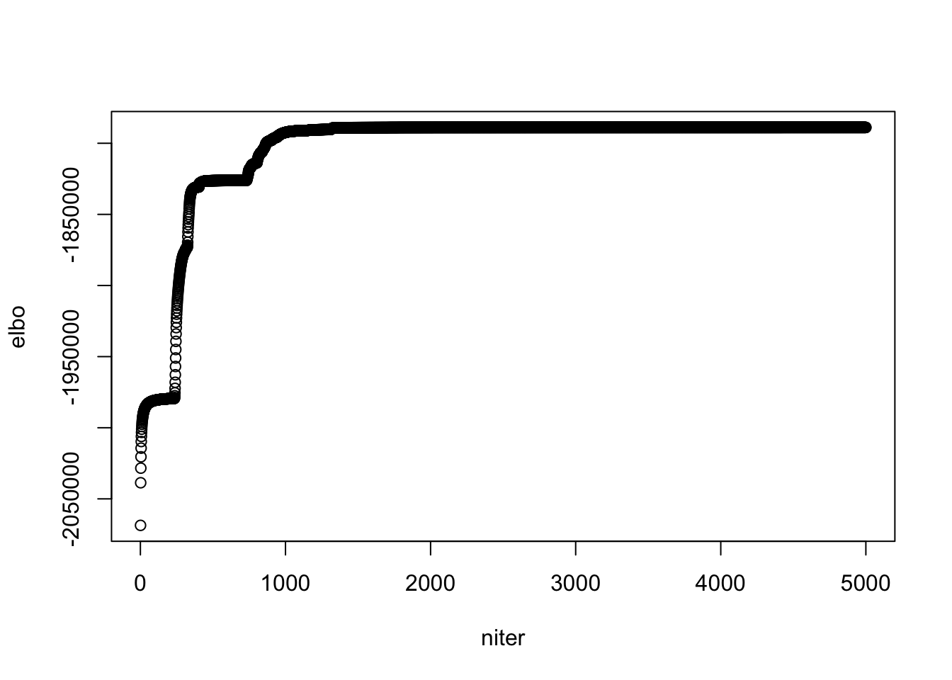
## runtime
model$runtime
user system elapsed
58135.647 49.558 37755.845 look at \(g_L, g_F\)
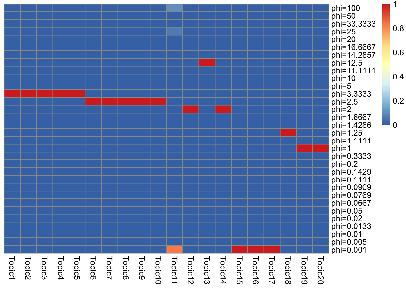
- I show component proportions for \(g_L, g_F\).
- It is interesting that almost all topics have only one component… (at iteration 500, all topic have one component). Is it because of initialization? Or is the discrete component truly a good global solution? (If that’s the case we can just do a grid search instead of solving a convex problem).
get_prior_summary <- function(gs){
  K = length(gs)
  phi_L = gs[[1]][["scale"]]
  idx = order(phi_L, decreasing = TRUE)
  L = length(phi_L)
  Pi = matrix(, nrow = L, ncol = K)
  for(k in 1:K){
    Pi[,k] = gs[[k]][["pi"]][idx]
  }
  rownames(Pi) = paste("phi=", round(phi_L[idx], digits = 4), sep = "")
  colnames(Pi) = paste("Topic", 1:K, sep = "")
  pheatmap(Pi, cluster_rows=FALSE, cluster_cols=FALSE)
}
\(g_L\)
get_prior_summary(model$qg$gls)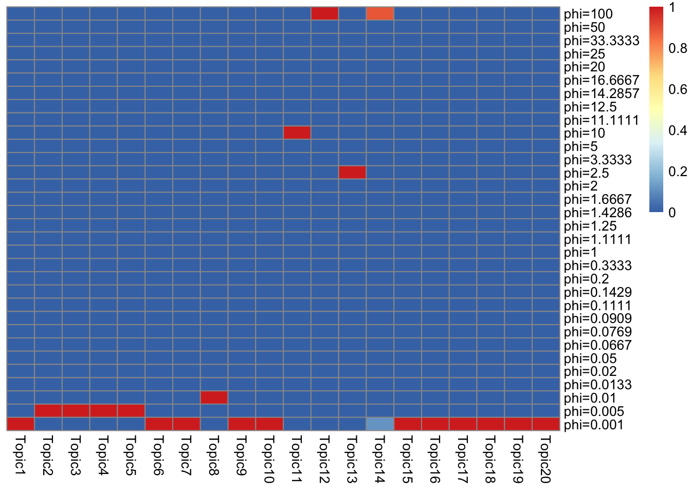
Some topics are almost the same.
- Note that a few \((l_k, f_k)\) pairs are very similar to each other (like the first 5 topics are almost identical). Below are the \(|\bar{f}_{J,2} - \bar{f}_{J,k}|_1, k = 1,3,4,5\) and \(|\bar{l}_{J,2} - \bar{l}_{J,k}|_1, k = 1,3,4,5\).
- Those almost identical topics/loadings are adjacent in our update order. It seems we need to randomize the update order?
print("|f_2 - f_k|_1, k = 1,3,4,5")[1] "|f_2 - f_k|_1, k = 1,3,4,5"f = model$qg$qfs_mean
sum(abs(f[,2] - f[,1]))[1] 1.941782sum(abs(f[,2] - f[,3]))[1] 1.042236e-07sum(abs(f[,2] - f[,4]))[1] 2.084468e-07sum(abs(f[,2] - f[,5]))[1] 3.126695e-07print("|l_2 - l_k|_1, k = 1,3,4,5")[1] "|l_2 - l_k|_1, k = 1,3,4,5"l = model$qg$qls_mean
sum(abs(l[,2] - l[,1]))[1] 3.230945sum(abs(l[,2] - l[,3]))[1] 3.03823e-10sum(abs(l[,2] - l[,4]))[1] 6.076523e-10sum(abs(l[,2] - l[,5]))[1] 9.114836e-10quantile of \(f_{J0}\)
f = model$f0
probs = seq(0, 1, 0.002)
plot(probs, quantile(f, probs = probs), main = sprintf("topic %d",0))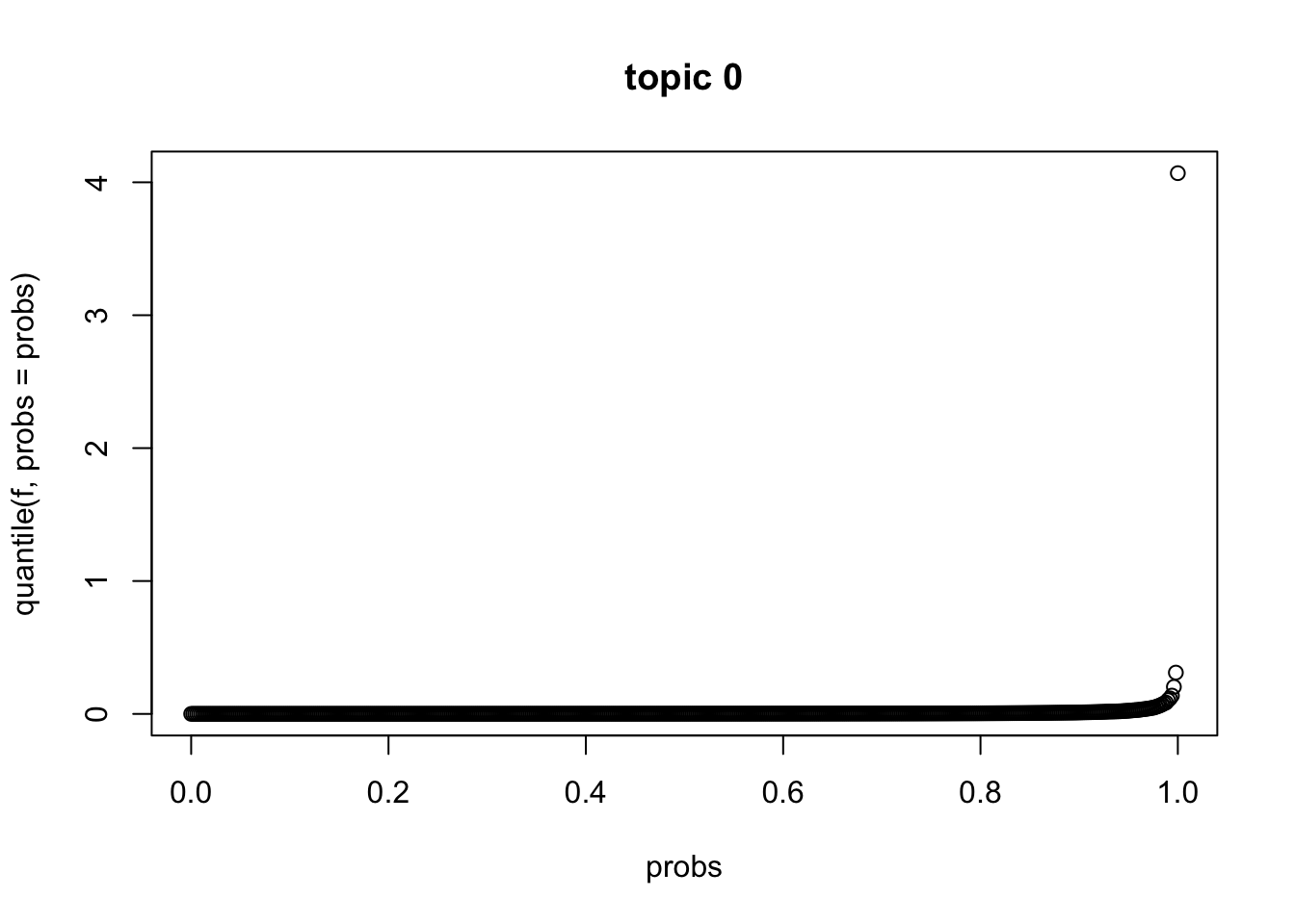
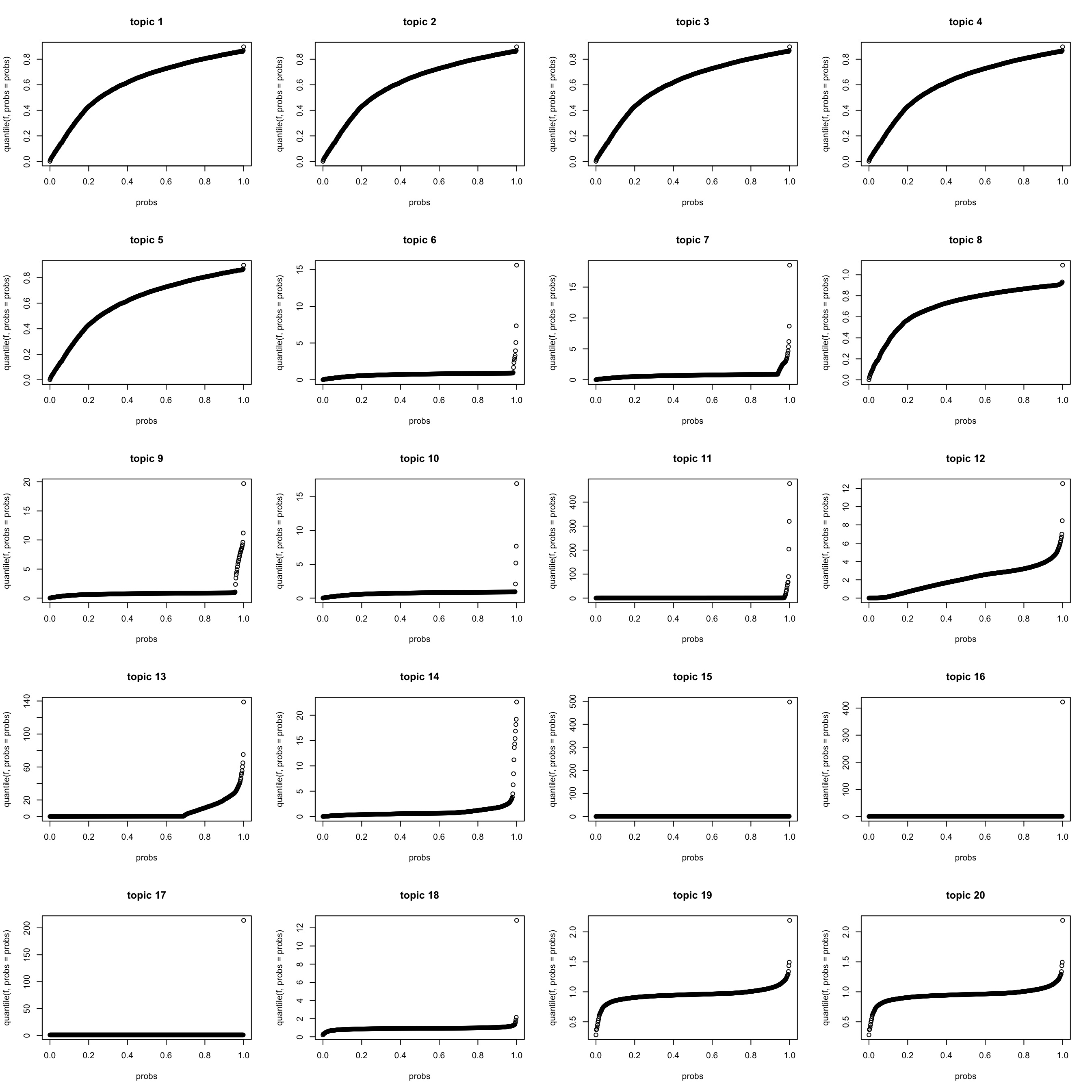
quantile of \(f_{Jk} (k > 0)\)
It seems that many topics contain lots of finer structure (not easily explained by a few words). This is not DIFFERENT from what we see from pNMF results.
K = length(model$qg$gls)
par(mfrow = c(5,4))
for(k in 1:K){
  f = model$qg$qfs_mean[,k]
  probs = seq(0, 1, 0.002)
  plot(probs, quantile(f, probs = probs), main = sprintf("topic %d",k))
}
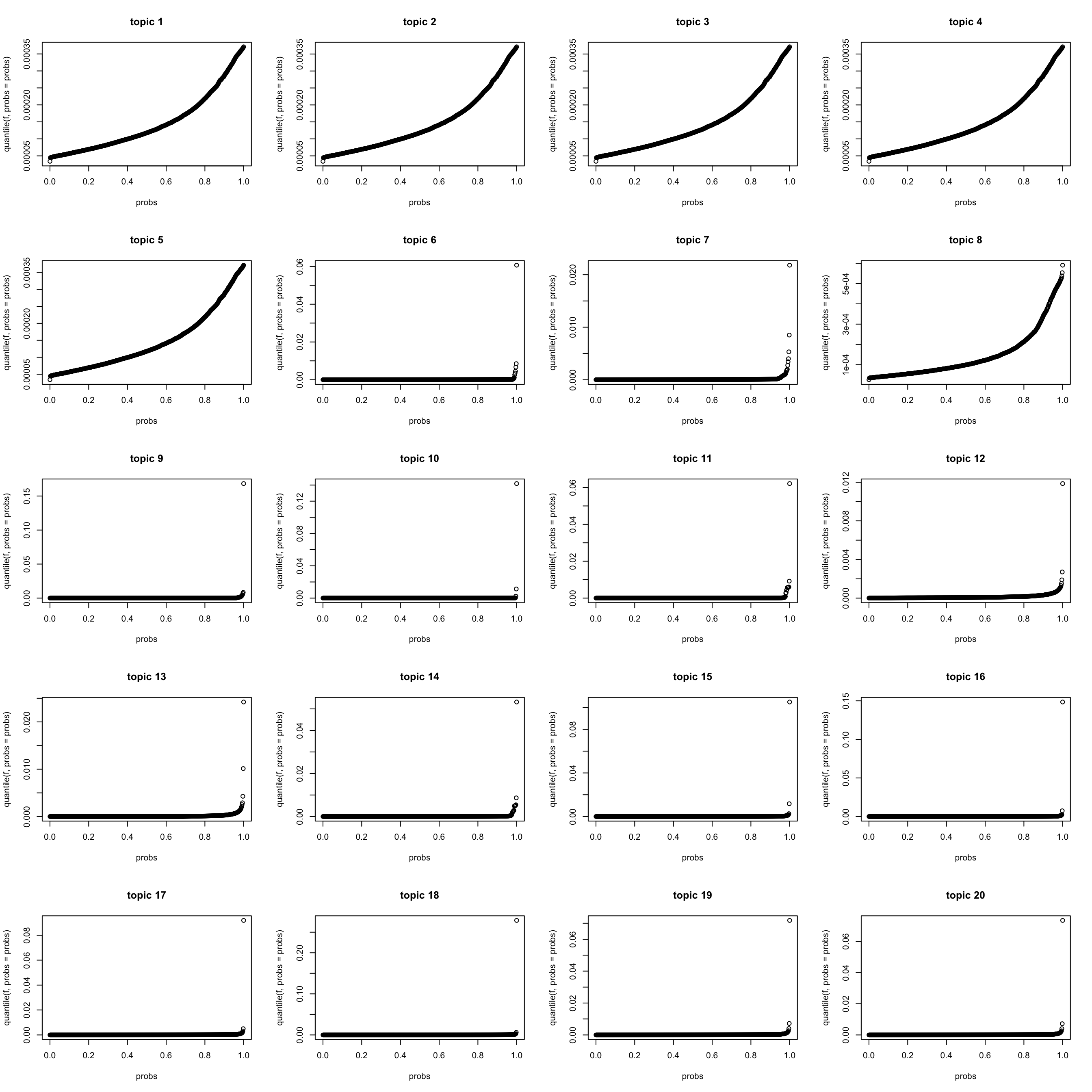
quantile of \(f_{J0} f_{Jk}\) (scaled to multinom model)
lf = poisson2multinom(F = model$f0 * model$qg$qfs_mean,
                 L = model$l0 * model$qg$qls_mean)

K = length(model$qg$gls)
par(mfrow = c(5,4))
for(k in 1:K){
  f = lf$F[,k]
  probs = seq(0, 1, 0.002)
  plot(probs, quantile(f, probs = probs), main = sprintf("topic %d",k))
}
| Version | Author | Date |
|---|---|---|
| 90f2fbd | zihao12 | 2020-05-12 |
look at \(s_k\)
\(s_k := \sum_i l_i0 \bar{l}_{ik}\). I make \(\sum_j f_{j0} = 1\) for interpretability.
d = sum(model$f0)
s_k = colSums(d * model$l0 * model$qg$qls_mean)
names(s_k) <- paste("Topic", 1:K, sep = "")
#round(s_k[1:5], digits = 0)
step = 5
for(i in 1:round(K/step)){
  print(round(s_k[((i-1)*step + 1):(i*step)]))
}
Topic1 Topic2 Topic3 Topic4 Topic5
5802 5791 5791 5791 5791
Topic6 Topic7 Topic8 Topic9 Topic10
6334 7757 5778 5812 5802
Topic11 Topic12 Topic13 Topic14 Topic15
7999 361414 15154 25447 5808
Topic16 Topic17 Topic18 Topic19 Topic20
5810 5807 5805 5805 5805 look at top words for topics
look at the top words in \(\bar{f}_{Jk}\).
K_sub <- 1:K
#par(mfrow = c(5,4))
p = length(model$l0)
n_top_word = round(0.002 * p)
f = model$qg$qfs_mean

show_topic <- function(k){
  #print(sprintf("topic %d", k))
  word_idx = order(f[,k], decreasing = TRUE)[1:n_top_word]
  F_sub = model$qg$qfs_mean[word_idx,]
  rownames(F_sub) = dict[word_idx]
  colnames(F_sub) = paste("Topic", 1:K, sep = "")
  pheatmap(F_sub,
           cluster_rows=FALSE, cluster_cols=FALSE,
           silent = TRUE,
           main = sprintf("topic %d", k))[[4]]
}
gs = lapply(K_sub, FUN = show_topic)
grid.arrange(grobs = gs, ncol = 4)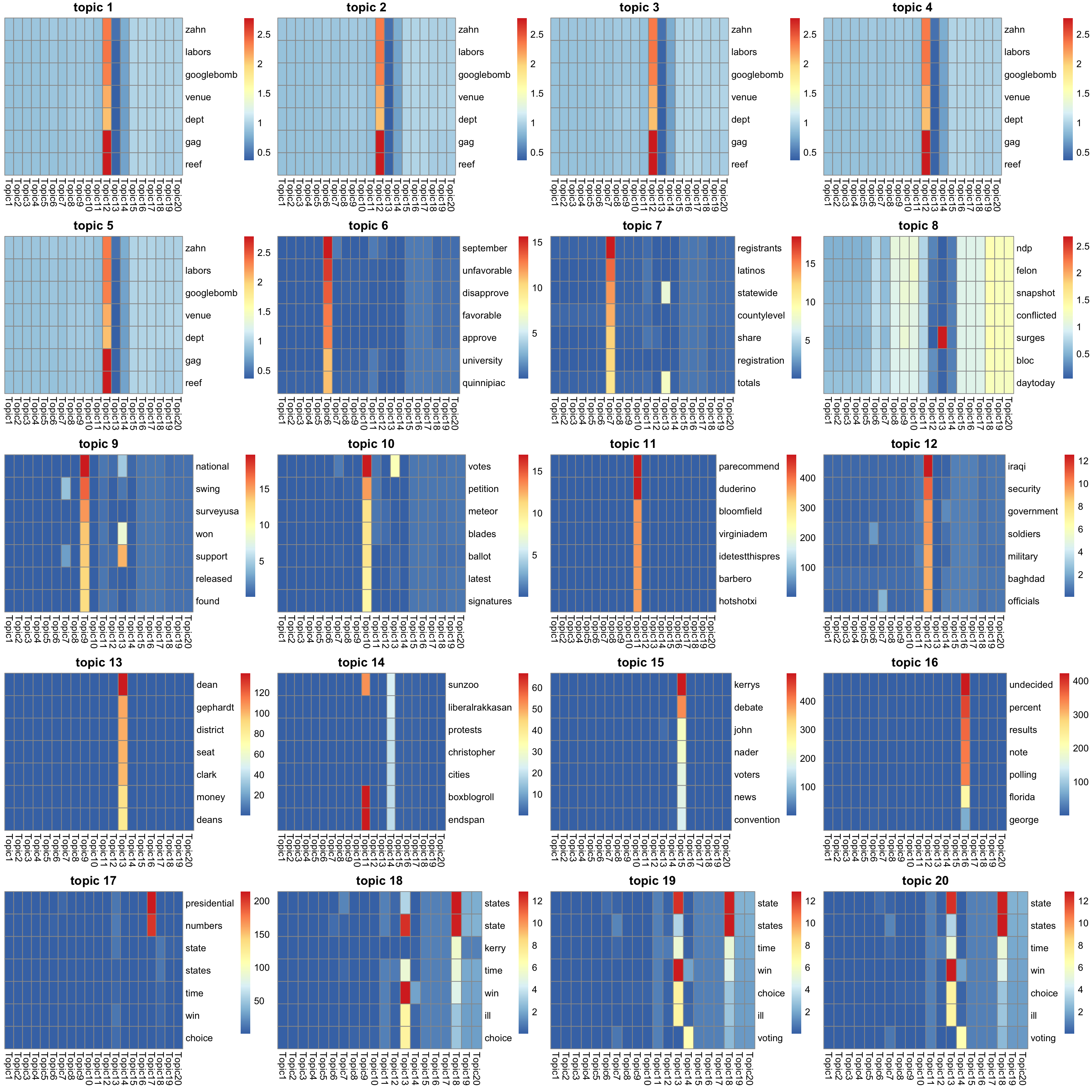
look at the top words in \(f_{J0}\bar{f}_{Jk}\) (after scaling to multinom model).
K_sub <- 1:K
#par(mfrow = c(5,4))
p = length(model$l0)
n_top_word = round(0.002 * p)
f = lf$F

show_topic <- function(k){
  #print(sprintf("topic %d", k))
  word_idx = order(f[,k], decreasing = TRUE)[1:n_top_word]
  F_sub = model$qg$qfs_mean[word_idx,]
  rownames(F_sub) = dict[word_idx]
  colnames(F_sub) = paste("Topic", 1:K, sep = "")
  pheatmap(F_sub,
           cluster_rows=FALSE, cluster_cols=FALSE,
           silent = TRUE,
           main = sprintf("topic %d", k))[[4]]
}
gs = lapply(K_sub, FUN = show_topic)
grid.arrange(grobs = gs, ncol = 4)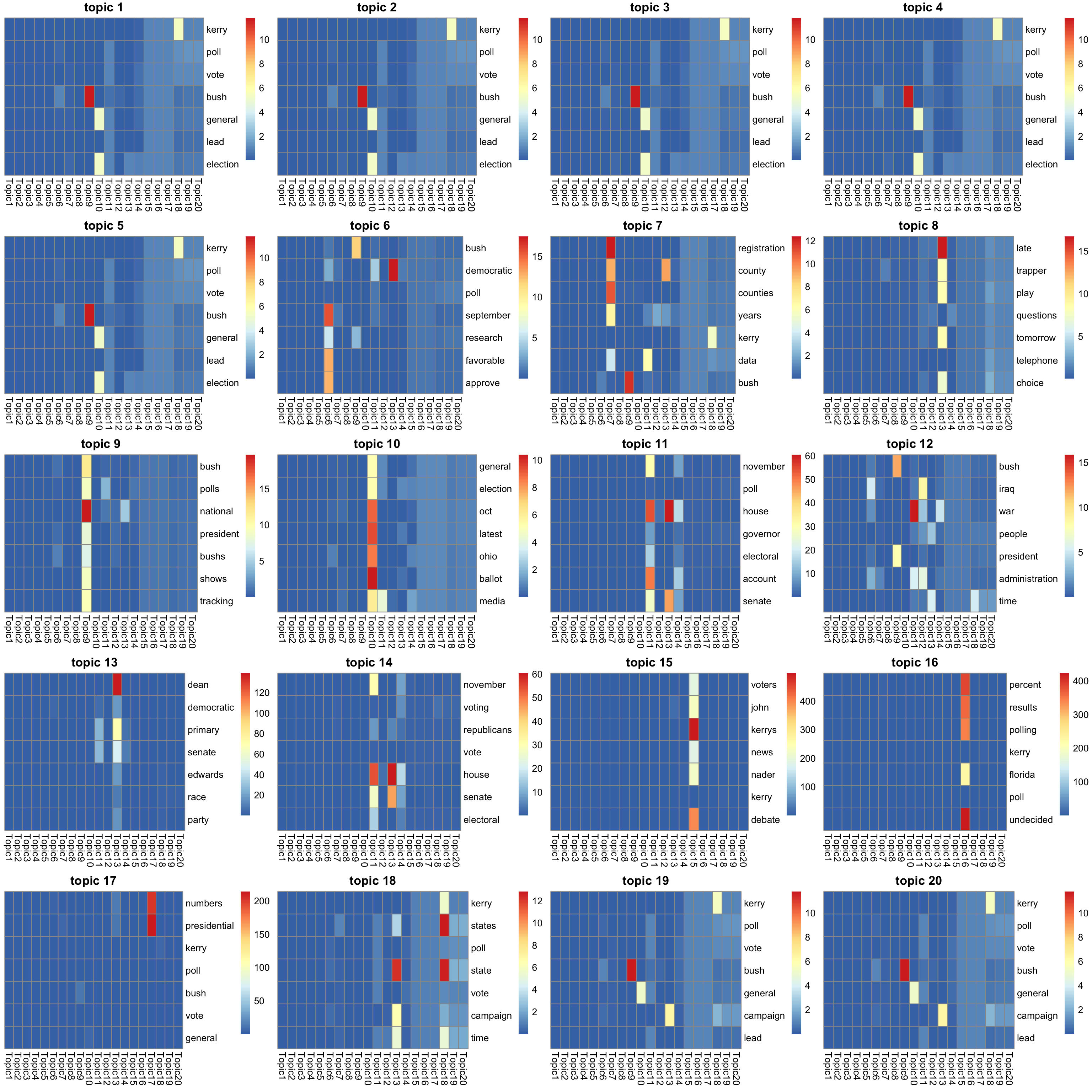
| Version | Author | Date |
|---|---|---|
| 90f2fbd | zihao12 | 2020-05-12 |
sessionInfo()R version 3.5.1 (2018-07-02)
Platform: x86_64-apple-darwin15.6.0 (64-bit)
Running under: macOS 10.14
Matrix products: default
BLAS: /Library/Frameworks/R.framework/Versions/3.5/Resources/lib/libRblas.0.dylib
LAPACK: /Library/Frameworks/R.framework/Versions/3.5/Resources/lib/libRlapack.dylib
locale:
[1] en_US.UTF-8/en_US.UTF-8/en_US.UTF-8/C/en_US.UTF-8/en_US.UTF-8
attached base packages:
[1] stats graphics grDevices utils datasets methods base
other attached packages:
[1] gridExtra_2.3 pheatmap_1.0.12
loaded via a namespace (and not attached):
[1] Rcpp_1.0.2 knitr_1.28 whisker_0.3-2 magrittr_1.5
[5] workflowr_1.6.2 munsell_0.5.0 colorspace_1.4-1 R6_2.4.0
[9] stringr_1.4.0 tools_3.5.1 grid_3.5.1 gtable_0.3.0
[13] xfun_0.8 git2r_0.26.1 htmltools_0.3.6 yaml_2.2.0
[17] digest_0.6.22 rprojroot_1.3-2 RColorBrewer_1.1-2 later_0.8.0
[21] promises_1.0.1 fs_1.3.1 glue_1.3.1 evaluate_0.14
[25] rmarkdown_2.1 stringi_1.4.3 compiler_3.5.1 scales_1.0.0
[29] backports_1.1.5 httpuv_1.5.1